Kinematics: the geometry of motion

Galileo’s Physics: Kinematics

Galileo Galilei 1564-1642, created the foundations for classical engineering physics by defining kinematics. Kinematics is the study of the geometry of motion. He observed the motion of planets, stars, falling objects, etc. Galileo defined used the relationships between position, velocity, and acceleration to make informed predictions.

One of the first kinematic experiments, was Galileo’s inclined ramp. Galileo’s hypthosis: objects all fall at the same rate of change in speed. Now, engineers take this for granted and use a gravitational constant to describe acceleration, \(g=9.81~\frac{m}{s^2}\).

Inclined ramp experiment

Placing two round objects, of the same shape, on an inclined plane, you can release them and see they both

• move the same distance in the same amount of time

• move slowly at first, then fastest at the end of the ramp

• the distance travelled is \(d \propto t^2\) time-squared

The last obeservation is harder to see, but if you use a stopwatch and meter stick you can create a table for distance and time.

Classical physics describes the position of an object using three independent coordinates e.g.

\[\mathbf{r}_{P/O} = x\hat{i} + y\hat{j} + z\hat{k}\]

where \(\mathbf{r}_{P/O}\) is the position of point \(P\) with respect to the point of origin \(O\), \(x,~y,~z\) are magnitudes of distance along a Cartesian coordinate system and \(\hat{i},~\hat{j}\) and \(\hat{k}\) are unit vectors that describe three

Show code cell content Hide code cell content

import numpy as np
import matplotlib.pyplot as plt
plt.style.use('fivethirtyeight')

Velocity

The velocity of an object is the change in () per length of time.

()\[\begin{equation} \mathbf{v}_{P/O} = \frac{d\mathbf{r}_{P/O}}{dt} = \dot{x}\hat{i} + \dot{y}\hat{j} + \dot{z}\hat{k} \end{equation}\]

Note: The notation \(\dot{x}\) and \(\ddot{x}\) is short-hand for writing out \(\frac{dx}{dt}\) and \(\frac{d^2x}{dt^2}\), respectively.

The definition of velocity in equation () depends upon the change in position of all three independent coordinates, where \(\frac{d}{dt}(x\hat{i})=\dot{x}\hat{i}\).

Example - GPS vs speedometer

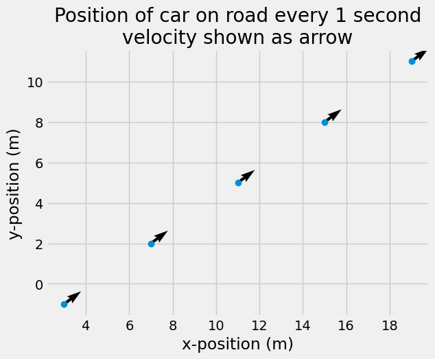
You can find velocity based upon postion, but you can only find changes in position with velocity. Consider tracking the motion of a car driving down a road using GPS. You determine its motion and create the position, \(\mathbf{r} = x\hat{i} +y\hat{j}\), where

\(x(t) = 4t + 3\) and \(y(t) = 3t - 1\)

To get the velocity, calculate \(\mathbf{v} = \dot{\mathbf{r}}\)

\(\mathbf{v} = 4\hat{i} +3 \hat{j}\)

Show code cell source Hide code cell source

t = np.arange(0,5)
x = 4*t + 3
y = 3*t -1
plt.plot(x,y,'o')
plt.quiver(x,y,4,3)
plt.title('Position of car on road every 1 second'+
    '\nvelocity shown as arrow')
plt.xlabel('x-position (m)')
plt.ylabel('y-position (m)');

Speed

The speed of an object is the magnitude of the velocity,

\(|\mathbf{v}_{P/O}| = \sqrt{\mathbf{v}\cdot\mathbf{v}} = \sqrt{\dot{x}^2 + \dot{y}^2 + \dot{z}^2}\)

Remember the chain rule

In Dynamics, there are many moving parts, so it is usually safer to assume that a variable is a function of time. Consider the derivative of position,

()\[\begin{equation} \frac{d}{dt}(x\hat{i}+y\hat{j}) = \dot{x}\hat{i} + \dot{y}\hat{j} + x\dot{\hat{i}} + y\dot{\hat{j}}, \end{equation}\]

in a fixed coordinate system (like the ground) \(\dot{\hat{i}}=\dot{\hat{j}}=0\) because these unit vectors do not change direction.

Chain rule in dynamics

In calculus, many times the chain rule is shown as an example

• \[\frac{d}{dx}(\sin x^2) = \frac{d}{dx}(x^2)\cdot \cos x^2\]
• \[\frac{d}{dx}(\sin x^2)= 2x\cos x^2\]

When you do this calculation, you have used the chain rule, but there is a hidden step multiplying by a chain rule operator $\(\frac{dx^2}{dx^2}\)$:

• \[\frac{d}{dx}(\sin x^2) = \frac{dx^2}{dx}\frac{d}{dx^2}\cdot \cos x^2\]
• \[\frac{d}{dx}(\sin x^2) = \frac{d}{dx}{x^2}\cdot\frac{d}{dx^2}(\cos x^2)\]
• \[\frac{d}{dx}(\sin x^2) = \frac{d}{dx}(x^2)\cdot \cos x^2\]
• \[\frac{d}{dx}(\sin x^2)= 2x\cos x^2\]

The chain rule in our case is used for functions of time, $\(t\)\( e.g. \)\(x(t),~y(t),~\theta(t)\)$

So, when you take a derivative of a function:

• \[\frac{d}{dt}\sin\theta = \frac{d\theta}{dt}\frac{d}{d\theta}\sin\theta\]
• \[\frac{d}{dt}\sin\theta =\frac{d\theta}{dt}\cos\theta\]
• \[\frac{d}{dt}\sin\theta =\dot{\theta}\cos\theta\]

Acceleration

The acceleration of an object is the change in velocity per length of time.

\(\mathbf{a}_{P/O} = \frac{d \mathbf{v}_{P/O} }{dt} = \ddot{x}\hat{i} + \ddot{y}\hat{j} + \ddot{z}\hat{k}\)

where \(\ddot{x}=\frac{d^2 x}{dt^2}\) and \(\mathbf{a}_{P/O}\) is the acceleration of point \(P\) with respect to the point of origin \(O\).

Rotation and Orientation

The definitions of position, velocity, and acceleration all describe a single point, but dynamic engineering systems are composed of rigid bodies is needed to describe the position of an object.

Show code cell source Hide code cell source

from IPython.core.display import SVG

SVG(filename='./images/position_angle.svg')

In the figure above, the center of the block is located at \(r_{P/O}=x\hat{i}+y\hat{j}\) in both the left and right images, but the two locations are not the same. The orientation of the block is important for determining the position of all the material points.

In general, a rigid body has a pitch, yaw, and roll that describes its rotational orientation, as seen in the animation below. We will revisit 3D motion in Module_05

Show code cell source Hide code cell source

from IPython.display import YouTubeVideo
vid = YouTubeVideo("li7t--8UZms?loop=1")
display(vid)

Rotation in planar motion

Our initial focus is planar rotations e.g. yaw and roll are fixed. For a body constrained to planar motion, you need 3 independent measurements to describe its position e.g. \(x\), \(y\), and \(\theta\)