Show code cell content Hide code cell content

import numpy as np
import matplotlib.pyplot as plt
from scipy.optimize import fsolve
plt.style.use('fivethirtyeight')

Module 3 - Project: pendulum solutions

In this notebook, you will compare two solutions for the motion of a swinging pendulum

1. linearized solution for \(\ddot{\theta}(t) = -\frac{g}{L}\theta\)

2. numerical solution for \(\ddot{\theta}(t) = -\frac{g}{L}\sin\theta\)

You can choose your own pendulum length \(L\) for the analysis. Try tying a string to an object and recording the swinging of the pendulum. You can estimate the initial angle and its period of oscillation.

1. Linear solution

The linear solution is the first order Taylor series approximation for the equation of motion

\(\ddot{\theta}(t) = -\frac{g}{L}\sin\theta \approx -\frac{g}{L}\theta\)

The solution to this simple harmonic oscillator function is

\(\theta(t) = \theta_0 \cos\omega t + \frac{\dot{\theta}_0}{\omega}\sin\omega t\)

where \(\theta_0\) is the initial angle, \(\dot{\theta}_0\) is the initial angular velocity [in rad/s], and \(\omega=\sqrt{\frac{g}{L}}\).

Here, you can plot the solution for

• \(L = 1~m\)

• \(g = 9.81~m/s^2\)

• \(\theta_0 = \frac{\pi}{3} = [60^o]\)

• \(\dot{\theta}_0 = 0~rad/s\)

g = 9.81 # m/s/s
L = 1 # m
w = np.sqrt(g/L) # rad/s
t = np.linspace(0, 4*np.pi/w) # 2 time periods of motion
theta0 = np.pi/3
dtheta0 = 0

theta = theta0*np.cos(w*t) + dtheta0/w*np.sin(w*t)

plt.plot(t, theta*180/np.pi)
plt.xlabel('time (s)')
plt.ylabel(r'$\theta(t)$ [degrees]')

Text(0, 0.5, '$\\theta(t)$ [degrees]')

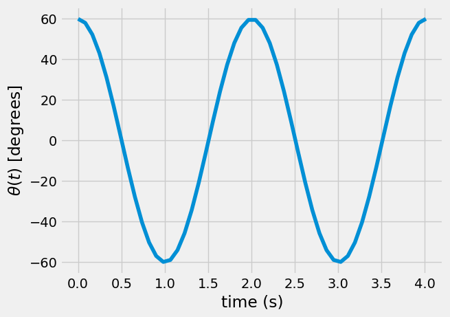
In the plot above, you should see harmonic motion. If it starts from rest at \(60^o\) the pendulum will swing to \(-60^o\) in \(\frac{T}{2} =\frac{\pi}{\omega}\) seconds.

2. Numerical solution

In the numerical solution, there is no need to linearize the equation of motion. You do need to create a state variable as such

\(\mathbf{x} = [x_1,~x_2] = [\theta,~\dot{\theta}]\)

now, you can describe 2 first order equations in a function as such

1. \(\dot{x}_1 = x_2\)

2. \(\dot{x}_2 = \ddot{\theta} =-\frac{g}{L}\sin\theta\)

putting this in a Python function it becomes

g = 9.81
L = 1
def pendulum(t, x):
    '''pendulum equations of motion for theta and dtheta/dt
    arguments
    ---------
    t: current time
    x: current state variable [theta, dtheta/dt]
    outputs
    -------
    dx: current derivative of state variable [dtheta/dt, ddtheta/ddt]'''
    
    dx = np.zeros(len(x))
    dx[0] = x[1]
    dx[1] = -g/L*np.sin(x[0])
    return dx

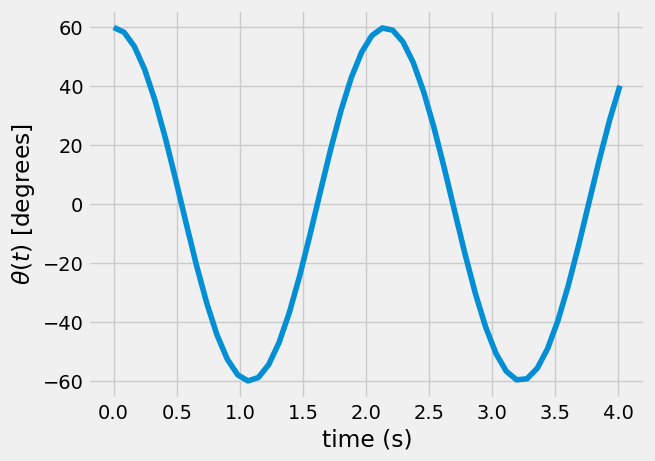
This function pendulum defines the differential equation. Next, integrate with solve_ivp to find \(\theta(t)\) as such.

Note: Here, I am using some previously defined values:

• theta0: the initial angle

• dtheta0: the initial angular velocity

• t: the timesteps from the previous linear analysis \(t = (0...2T)\)

Show code cell source Hide code cell source

from scipy.integrate import solve_ivp

sol = solve_ivp(pendulum, [0, t.max()], [theta0, 0], t_eval = t)
plt.plot(sol.t, sol.y[0]*180/np.pi)
plt.xlabel('time (s)')
plt.ylabel(r'$\theta(t)$ [degrees]')

Text(0, 0.5, '$\\theta(t)$ [degrees]')

Comparing results

At first glance, it would seem both solutions are close enough, but here you can plot them together and compare.

plt.plot(t, theta*180/np.pi)
plt.plot(sol.t, sol.y[0]*180/np.pi)
plt.xlabel('time (s)')
plt.ylabel(r'$\theta(t)$ [degrees]')

Text(0, 0.5, '$\\theta(t)$ [degrees]')

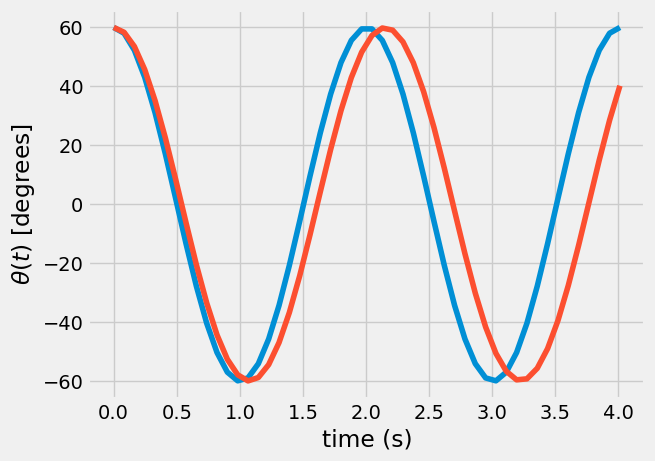
You should notice a difference in time period between the two solutions, which means the natural frequencies are different.

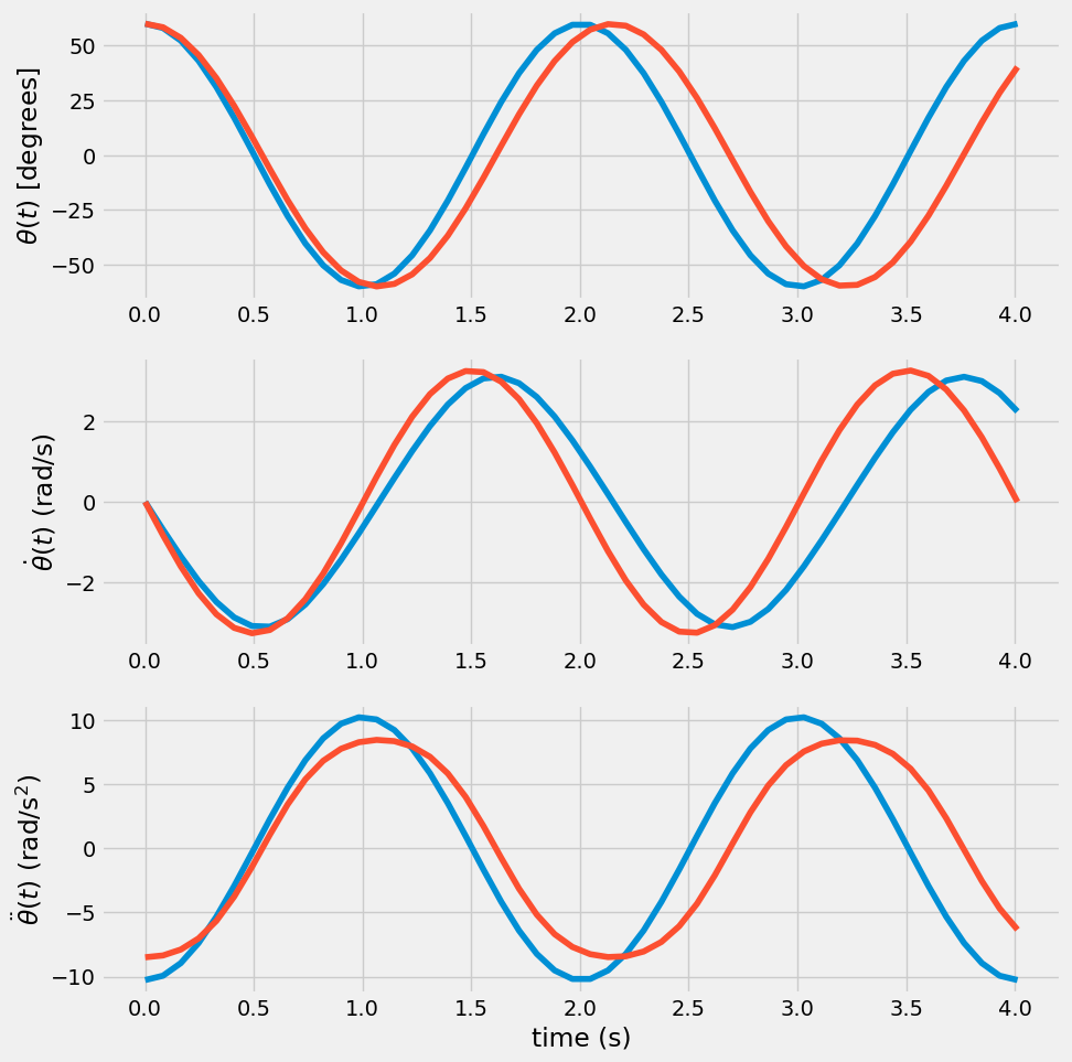
You can also consider angular velocity and angular acceleration, below a set of 3 plots are shown for \(\theta(t),~\dot{\theta}(t),~and~\ddot{\theta}(t)\).

dtheta = -theta0*w*np.sin(w*t) + dtheta0*np.cos(w*t)
ddtheta = -theta0*w**2*np.cos(w*t) - dtheta0*w*np.sin(w*t)

ddtheta_numerical = -g/L*np.sin(sol.y[0]) # using equation of motion

plt.figure(figsize= (10, 11))
plt.subplot(311)
plt.plot(t, theta*180/np.pi)
plt.plot(sol.t, sol.y[0]*180/np.pi)

plt.ylabel(r'$\theta(t)$ [degrees]')

plt.subplot(312)
plt.plot(sol.t, sol.y[1])
plt.plot(t, dtheta)

plt.ylabel(r'$\dot{\theta}(t)$ (rad/s)')


plt.subplot(313)
plt.plot(t, ddtheta)
plt.plot(t, ddtheta_numerical)
plt.xlabel('time (s)')
plt.ylabel(r'$\ddot{\theta}(t)$ (rad/s$^2$)')

Text(0, 0.5, '$\\ddot{\\theta}(t)$ (rad/s$^2$)')

Question prompt

• Where do you see the biggest difference between the linearized solution and the numerical solution?

• What are ways you can quantify the error between then two results? Is one solution more accurate?

• What other calculations can you compare between these two solutions?