Kinematics in cylindrical coordinates#

It helps to see the motion to understand what’s going on, the position of the ball is

$\mathbf{r}=x\hat{i}+y\hat{j}=r(\cos \theta \hat{i}+\sin \theta \hat{j})$

while its velocity and acceleration are represented in cylindrical coordinates

• $\mathbf{v}=\dot{x}\hat{i}+\dot{y}\hat{j}=\dot{r}{\hat{e}}_r+r\dot{\theta }{\hat{e}}_{\theta }$

• $\mathbf{a}=\ddot{x}\hat{i}+\ddot{y}\hat{j}=(\ddot{r}-r{\dot{\theta }}^2){\hat{e}}_r+(r\ddot{\theta }+2\dot{r}\dot{\theta }){\hat{e}}_{\theta }$

Kinetics of central spring force#

The free body diagram has a single central spring force and the kinetic diagram include radial $a_r$ and transverse $a_{\theta }$ acceleration components, but no moment is applied

1. $\sum F_r=-k(r-L_0)=m(\ddot{r}-r{\dot{\theta }}^2)$

2. $\sum F_{\theta }=0=m(r\ddot{\theta }+2\dot{r}\dot{\theta })$

3. $\sum M_O=0=\frac{d}{dt}\left(m{r}^2\dot{\theta }\right)$

Equation of motion for central spring force#

Combining equations 1&3, you have a single, second order differential equation that describes radius as a function of time, $r(t)$

$\ddot{r}=-\frac{k}{m}(r-L_0)+\frac{r_0^4{\dot{\theta }}_0^2}{r^3}$

where $r_0$ is the initial radius and ${\dot{\theta }}_0$ is the initial angular velocity.

Initial conditions due to Impulse#

When an impulse, $F\mathrm{\Delta }t$, is applied to a dynamic system, you have an instantaneous change in momentum

$F\mathrm{\Delta }t=\mathrm{\Delta }mv$.

It also creates a moment to create the initial angular momentum

$M\mathrm{\Delta }t=\mathrm{\Delta }{\mathbf{h}}_O(t=0)$

The impulse is gone after that initial impact. It gives you the initial conditions of velocity and angular momentum,

• $\mathbf{v}(t=0)=v_0(\sin {45}^o\hat{i}+\cos {45}^o\hat{j})=\dot{r}{\hat{e}}_r+r\dot{\theta }{\hat{e}}_{\theta }$

• ${\mathbf{h}}_O(t=0)=m{L}_0{v}_0\cos {45}^o=m{r}_0^2{\dot{\theta }}_0$

Total solution and animation#

Now, you have

1. equation of motion in terms of $rand\ddot{r}$

2. initial conditions, $r(t=0)=L_{0}and\dot{r}(t=0)=\frac{v_O}{\sqrt{2}}$

So you can create a differential equation and integrate using the solve_ivp

import numpy as np
import matplotlib.pyplot as plt
plt.style.use('fivethirtyeight')
from scipy.integrate import solve_ivp

Here, you set up constants

• spring constant k in N/m

• unstretched spring length L0 in m

• mass of ball m in kg

• initial speed v0 in m/s note: the direction is at a 45${}^o$ angle

and define the differential equation in 2 steps:

1. dr[0] = r[1] states $dr/dt=\dot{r}$

2. dr[1] = -k/m*(r[0] - L0) +r[0]*(L0*v0/r[0])**2/2 gives the equation of motion solved for $\ddot{r}$

k = 100
L0 = 0.5
m = 0.5
v0 = 5

def my_ode(t, r):
    dr = np.zeros(len(r))
    dr[0] = r[1]
    dr[1] = -k/m*(r[0] - L0) +r[0]*(L0*v0/r[0])**2/2
    return dr

Integrate the equation of motion by using

• timespan 0 to tend

• initial conditions $r(t=0)=L_{0}and\dot{r}(t=0)=\frac{v_0}{\sqrt{2}}$ as [L0, v0/2**0.5]

• sol = solve_ivp integrates the equation of motion

the output for sol includes

• timesteps sol.t

• radius, $r(t)$ sol.y[0]

• radial velocity, $\dot{r}(t)$ sol.y[1]

tend = 3
r0 = np.array([L0, v0/2**0.5])
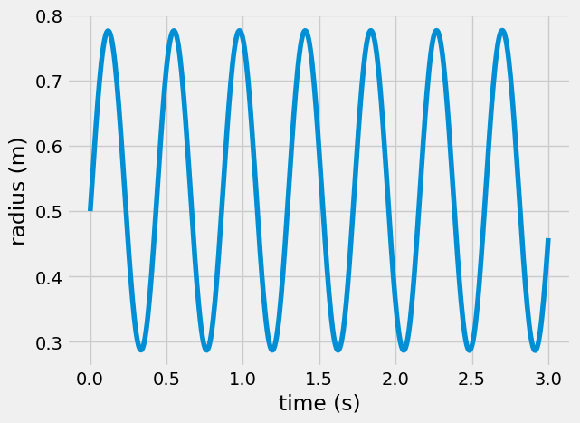
sol = solve_ivp(my_ode, [0, tend], r0, t_eval = np.linspace(0, tend, 500))
plt.plot(sol.t, sol.y[0])
plt.xlabel('time (s)')
plt.ylabel('radius (m)')

Text(0, 0.5, 'radius (m)')

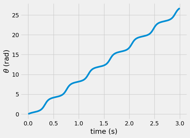
You don’t have an equation for $\theta (t)$, but you can use angular momentum to calculate $\dot{\theta }$

$\dot{\theta }(t)=\frac{h_O(t=0)}{r^2}$

then, the solution for $\theta =\sum \dot{\theta }dt$ or np.cumsum(dtheta*sol.t[1]) - theta[0]

dtheta = L0*v0/2**0.5/sol.y[0]**2
theta = np.cumsum(dtheta*sol.t[1])
theta += -theta[0]
plt.plot(sol.t, theta)
plt.xlabel('time (s)')
plt.ylabel(r'$\theta$ (rad)')

Text(0, 0.5, '$\\theta$ (rad)')

Finally, you can get the $r-\theta$ coordinates back into $x-y$ coordinates and animate the motion

x = sol.y[0]*np.cos(theta)
y = sol.y[0]*np.sin(theta)

Show code cell content Hide code cell content

from matplotlib import animation
from IPython.display import HTML

fig, ax = plt.subplots()

#ax.set_xlim(( -30, 30))
# ax.set_ylim((1.5, -1.5))
ax.axis('equal')
ax.set_xlabel('x-position (m)')
ax.set_ylabel('y-position (m)')

line1, = ax.plot([], [],'-o')
line2, = ax.plot(x, y,'g--', alpha=0.5)

def init():
    line1.set_data([], [])
    line2.set_data([], [])
    return (line1, line2, )

def animate(i):
    '''function that updates the line and marker data
    arguments:
    ----------
    i: index of timestep
    outputs:
    --------
    line: the line object plotted in the above ax.plot(...)
    '''
    line1.set_data([0, x[i]], [0, y[i]])
    line2.set_data(x[0:i], y[0:i])
    return (line1, line2, )

anim = animation.FuncAnimation(fig, animate, init_func=init,
                               frames=range(0,len(sol.t)), interval=50, 
                               blit=True)

HTML(anim.to_html5_video())

---------------------------------------------------------------------------
RuntimeError                              Traceback (most recent call last)
Cell In[7], line 1
----> 1 HTML(anim.to_html5_video())

File /opt/hostedtoolcache/Python/3.9.21/x64/lib/python3.9/site-packages/matplotlib/animation.py:1265, in Animation.to_html5_video(self, embed_limit)
   1262 path = Path(tmpdir, "temp.m4v")
   1263 # We create a writer manually so that we can get the
   1264 # appropriate size for the tag
-> 1265 Writer = writers[mpl.rcParams['animation.writer']]
   1266 writer = Writer(codec='h264',
   1267                 bitrate=mpl.rcParams['animation.bitrate'],
   1268                 fps=1000. / self._interval)
   1269 self.save(str(path), writer=writer)

File /opt/hostedtoolcache/Python/3.9.21/x64/lib/python3.9/site-packages/matplotlib/animation.py:128, in MovieWriterRegistry.__getitem__(self, name)
    126 if self.is_available(name):
    127     return self._registered[name]
--> 128 raise RuntimeError(f"Requested MovieWriter ({name}) not available")

RuntimeError: Requested MovieWriter (ffmpeg) not available

Wrapping up#

In this notebook, you used conservation of angular momentum and Newton’s second law to create an equation of motion for the radius of a spring-mass stationary table. Then, you plotted the results and watched the path of the object over time.

Next steps:

• What happens if you change the parameters of the system, $k,L0,etc.$?

• What happens if you change the initial impulse applied to the ball?