Snowflake time of flight#
Have you ever watched a snowflake fall and thought, “How long has that snowflake been falling?”
Here, we want to determine the time of flight for a snowflake. We’ll start simple and add some complexity to make a more accurate model.
Simplest model#
The simplest assumption we can make is that the only force acting on the snowflake is gravity. This leads to one differential equation,
\(-mg = m\ddot{y}\)
where \(m\) is the mass of the snowflake, \(g=9.81~\frac{m}{s^2}\), and \(\ddot{y}\) is the second derivative with respect to time for the height of the snowflake i.e. its vertical acceleration.
We integrate this equation twice to create a solution in terms of \(y_0\), initial height and \(\dot{y}_0\), its initial vertical velocity.
\(\ddot{y} = -g\)
\(\frac{d\dot{y}}{dt} = -g\)
\(\dot{y} -\dot{y}_0 = -gt\)
\(\frac{dy}{dt} = \dot{y}_0 -gt\)
\(y-y_0 = \dot{y}_0t - \frac{gt^2}{2}\)
\(y(t) = y_0 +\dot{y}_0t - \frac{gt^2}{2}\)
Now, we need the initial height and initial speed of the snowflake. A typical cloud might sit \(\approx 1,000~m\) above the ground and let’s assume the initial vertical speed is 0 m/s.
This leaves, \(y_0=1000~m~and~\dot{y}_0=0~m/s\)

Text(0, 0.5, 'height (m)')
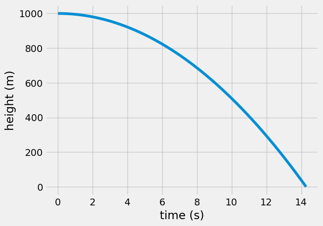
np.float64(14.278431229270645)
Our solution - constant acceleration#
According to your calculations, the snowflake will start at 1,000-m altitude and reach ground level at almost 14.3 seconds.
Note: What’s wrong with the height curve here?
A little problem - speed of snowflake#
The graph of height-vs-time keeps getting steeper. The steeper the graph, the faster the snowflake. How fast is your snowflake traveling when it hits the ground?
Text(0, 0.5, 'vertical speed (m/s)')
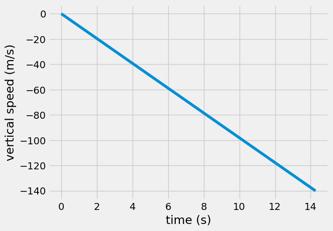
According to your calculations, the snowflake is traveling at 140 m/s when it strikes the ground. This is >300 mph (or >500 km/h). Whoah…
If you caught this snowflake on your tongue it would feel like catching an icy BB gun pellet, ouch!
You are missing a key force in the free body diagram that slows down the snowflake, air resistance or drag.
Improved model with air resistance#
Adding drag to the free body diagram, now you have a new model.
\(m\ddot{y} = -mg + C_d \frac{r\dot{y}^2}{2}A\)
where \(C_d\) is the unitless drag coefficient, \(r=1.025~kg/m^3\) is the density of air, \(m=3~mg\) is the mass of a snowflake, and \(A=\pi D^2/4\) is the area of the snowflake of diameter \(D=6~mm\).
Note: The force of drag always opposes the velocity of the snowflake. Keep in mind if the snowflake moves upward, the force reverses direction.
Now, integrating the equation can be a bit involved, but using v(t=0)=0, there results
\(\frac{dv}{dt} = -g +\frac{C_d rA}{2}v^2\)
\(v(t) = -\sqrt{\frac{mg}{C_d rA}}\tanh\frac{g C_d rA}{m}t\)
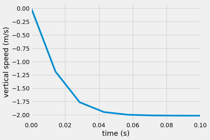
Text(0, 0.5, 'vertical speed (m/s)')
Make a comparison to previous model#
In the constant acceleration model, the snowflake reached the ground in 14 seconds. In the improved air resistance model, you find that the snowflake only accelerates for 0.5 seconds. After that, it floats at a constant velocity until impact. This means, you can approximate that the snowflake travels at a constant velocity equal to its terminal velocity, \(v_{term}\), as such
\(\frac{dv}{dt} = 0 = -g +\frac{C_d rA}{2m}v_{term}^2\)
\(v_{term} = -\sqrt{\frac{2mg}{C_d rA}}\)
total flight time is 496.1728506287249
Text(0, 0.5, 'height (m)')
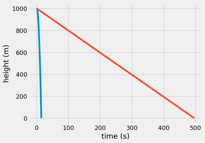
Wrapping up#
The first model you created assumed constant acceleration, but after accounting for drag you found out that a snowflake reaches a terminal velocity in less than 0.5 seconds. The more accurate model to calculate time of flight was actually a constant velocity model.
You found that the snowflake drifts slowly to the surface over the course of 496 seconds (or 8 minutes). Gently landing at 2 m/s.