Module 2 - Project: four-bar linkage design

Module 2 - Project: four-bar linkage design#

In this notebook, you will build your own four-bar mechanical linkage and plot the path of the components. You can choose your own link sizes. Some areas of interest for different backgrounds:

Automotive design: windshield wiper motion, watt linkage suspension
biomechanics: ACL-PCL knee joint model and knee replacement
anything else?

In this notebook, you will step through the process of defining the kinematics of a four-bar linkage.

What you’ll do#

solve a series of nonlinear equations using fsolve
use solutions to create 2D arrays that vary in time and location
plot and animate the motion of the four-bar linkage

What you’ll need#

Jupyter and Python - you can run this notebook with the “Launch” icon in the Engineering Dynamics online resource
vector equations to solve for the constraints on the linkage mechanism
A mechanical system to consider: choose three link lengths and the relative mounting position between the two
some plots and background explanation to explain what your mechanism is supposed to do

Diagram of a general four-bar linkage

\(l_1\sin\theta_1+l_2\sin\theta_2-l_3\sin\theta_3 -d_y = 0\)
\(l_1\cos\theta_1+l_2\cos\theta_2-l_3\cos\theta_3 -d_x = 0\)

If you have one of the angles, e.g. \(\theta_1\), you use equations 1 and 2 to solve for the other two angles, \(\theta_2~and\theta_3\). Here you can create a function and use fsolve. The function input is a vector with two values and the output is a vector with two values.

\(\bar{f}(\bar{x})= \left[\begin{array}{c} f_1(\theta_2,~\theta_3) \\ f_2(\theta_2,~\theta_3)\end{array}\right]=\left[\begin{array}{c} l_1\sin\theta_1+l_2\sin\theta_2-l_3\sin\theta_3 -d_y\\ l_1\cos\theta_1+l_2\cos\theta_2-l_3\cos\theta_3 -d_x \end{array}\right]\)

Defining your system#

As an example, I am creating a short arm that pivots a longer arm. Similar to a windshield wiper design

Note: you can double-click this cell in Jupyter to edit the text. Then, you can update the geometry of your four-bar linkage.

link 1: \(l_1 = 0.25~m\)
link 2: \(l_2 = 1~m\)
link 3: \(l_3 = 1~m\)
support: \(d_x=0.95~m~and~d_y=0~m\)

The constraint function is defined below as Fbar, a function of \(\theta_1\) and an array of \([\theta_2,~\theta_3]\) as such,

l1 = 0.25
l2 = 1
l3 = 1
a1 = np.pi/2
dy = 0
dx = 0.95
Fbar = lambda a1,x: np.array([l1*np.sin(a1)+l2*np.sin(x[0])-l3*np.sin(x[1])-dy,
                           l1*np.cos(a1)+l2*np.cos(x[0])-l3*np.cos(x[1])-dx])

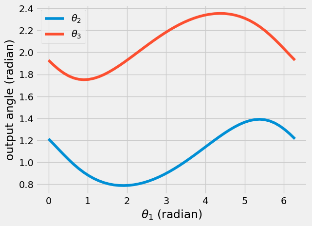
Next, I choose a range of motion for link 1

\(\theta_1 = (0,~2\pi) = (0,~360^o)\)

and solve for the angles of links 2 and 3 as such

initialize my variables a1 as \(0-2\pi\), a2 as zeros, a3 as zeros
set an initial solution guess for fsolve
use a for-loop to solve for a2 and a3 at each configuration

a1 = np.linspace(0, 2*np.pi)
a2 = np.zeros(len(a1))
a3 = np.zeros(len(a1))
xsol = np.array([0, np.pi/4])
for i in range(len(a1)):
    xsol = fsolve(lambda x: Fbar(a1[i], x), xsol)
    a2[i] = xsol[0]
    a3[i] = xsol[1]

plt.plot(a1, a2, label = r'$\theta_2$')
plt.plot(a1, a3, label = r'$\theta_3$')
plt.xlabel(r'$\theta_1$ (radian)')
plt.ylabel('output angle (radian)')
plt.legend();

../_images/9cfe03360588e91b6a47d0a18e9c5435f7543992e8462a88cd2acd6dc14d3ea7.png

Motion of the links#

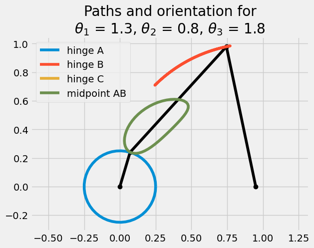
Now I have the position of the links, but I want to see what it looks like and what paths the components trace. Here, I use the vector definitions to define the positions of the links and connections

\(r_A = l_1 \cos\theta_1\hat{i} + l_1 \sin\theta_1\hat{j}\)
\(r_B = r_A + r_{B/A} = r_A + l_2\cos\theta_2\hat{i} + l_2 \sin\theta_2\hat{j}\)
\(r_C = r_B + r_{C/B} = r_B - l_3\cos\theta_3\hat{i} - l_3 \sin\theta_3\hat{j}\)
\(r_P = r_A + r_{P/A} = r_A + \frac{l_2}{2}\cos\theta_2\hat{i} + \frac{l_2}{2} \sin\theta_2\hat{j}\)

rA = l1*np.vstack([np.cos(a1), np.sin(a1)])
rB = rA + l2*np.vstack([np.cos(a2), np.sin(a2)])
rC = rB - l3*np.vstack([np.cos(a3), np.sin(a3)])
rP = rA + l2/2*np.vstack([np.cos(a2), np.sin(a2)])

Plot one orientation and the paths#

The paths of the links are now in the variables rA, rB, rC, and rP. I will plot the paths of these 4 points and the shape at a point in time.

links_x_locations = np.vstack([np.zeros(len(a1)), 
                              rA[0, :],
                              rB[0, :],
                              rC[0, :]])

links_y_locations = np.vstack([np.zeros(len(a1)), 
                              rA[1, :],
                              rB[1, :],
                              rC[1, :]])
i = 10
plt.plot(links_x_locations[:, i], 
        links_y_locations[:, i], 'k-o')
plt.plot(rA[0,:], rA[1,:], label = 'hinge A')
plt.plot(rB[0,:], rB[1,:], label = 'hinge B')
plt.plot(rC[0,:], rC[1,:], label = 'hinge C')
plt.plot(rP[0,:], rP[1,:], label = 'midpoint AB')
plt.legend()
plt.title('Paths and orientation for\n'+ 
          r'$\theta_1$ = {:.1f}, $\theta_2$ = {:.1f}, $\theta_3$ = {:.1f}'.format(a1[i], a2[i], a3[i]))
plt.axis('equal');

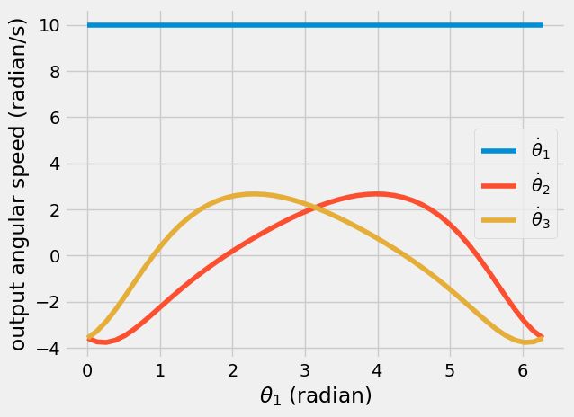
../_images/d6b69906e2831937943c345b3eff5c37da1f28c210355a6b14fe03fd03010d5e.png

Determining the speed of the components#

Now, I use the constraint equations from above to determine the speed of the link motion.

\(\frac{d\bar{f}(\bar{x})}{dt}= \left[\begin{array}{c} f_1(\theta_2,~\theta_3) \\ f_2(\theta_2,~\theta_3)\end{array}\right]=\left[\begin{array}{c} l_1\dot{\theta_1}\cos\theta_1+l_2\dot{\theta_2}\cos\theta_2-l_3\dot{\theta_3}\cos\theta_3\\ l_1\dot{\theta_1}\sin\theta_1+l_2\dot{\theta_2}\sin\theta_2-l_3\dot{\theta_3}\sin\theta_3 \end{array}\right]\)

define the 2-equation function
initialize the solutions for the arrays: da1, da2, da3
solve the equations at each step in time in a for-loop

drive_rate = 10 #rad/s
dFbar = lambda a1, a2, a3, dx: np.array([l1*drive_rate*np.sin(a1)+\
                                         l2*dx[0]*np.sin(a2)-\
                                         l3*dx[1]*np.sin(a3),\
                                         l1*drive_rate*np.cos(a1)+\
                                         l2*dx[0]*np.cos(a2)-\
                                         l3*dx[1]*np.cos(a3)])

da1 = np.ones(len(a1))*10
da2 = np.zeros(len(a1))
da3 = np.zeros(len(a1))
xsol = np.array([0, 0])


for i in range(len(a1)):
    xsol = fsolve(lambda dx: dFbar(a1[i], a2[i], a3[i], dx), xsol)
    da2[i] = xsol[0]
    da3[i] = xsol[1]

plt.plot(a1, da1, label = r'$\dot{\theta}_1$')
plt.plot(a1, da2, label = r'$\dot{\theta}_2$')
plt.plot(a1, da3, label = r'$\dot{\theta}_3$')
plt.legend()
plt.xlabel(r'$\theta_1$ (radian)')
plt.ylabel('output angular speed (radian/s)')

Text(0, 0.5, 'output angular speed (radian/s)')

../_images/bc601f662b2838bfc3b4ff705b26a6fcda24981bc2d5509941839cf7694d6697.png

Wrapping up#

You should edit this notebook to create your own four-bar linkage analysis.

Choose a geometry
plot the motion and paths
plot the speeds of the links
add your own wrapping up section to add any details or further analysis
what did you learn?