import numpy as np
import matplotlib.pyplot as plt
from scipy.optimize import fsolve
plt.style.use('fivethirtyeight')

Show code cell source Hide code cell source

from IPython.lib.display import YouTubeVideo
YouTubeVideo('Je-qT2FQrrM')

Solving equations of motion

In this notebook, you will plot the solutions to three 1-DOF equations of motion. Each starts at the origin with an initial velocity, \(v = 5~m/s\). The three equations of motion and solutions are derived in the video above

system	equation of motion	solution
a.	\(m\ddot{x} = -\mu mg\)	\(\rightarrow x(t) = v_0t - \frac{\mu gt^2}{2}\)
b.	\(m\ddot{x} = -b \dot{x}\)	\(\rightarrow x(t) = \frac{v_0 m}{b}\left(1 - e^{-\frac{b}{m} t}\right)\)
c.	\(m\ddot{x} = -k x\)	\(\rightarrow x(t) = \frac{v_0}{\omega}\sin\omega t\)

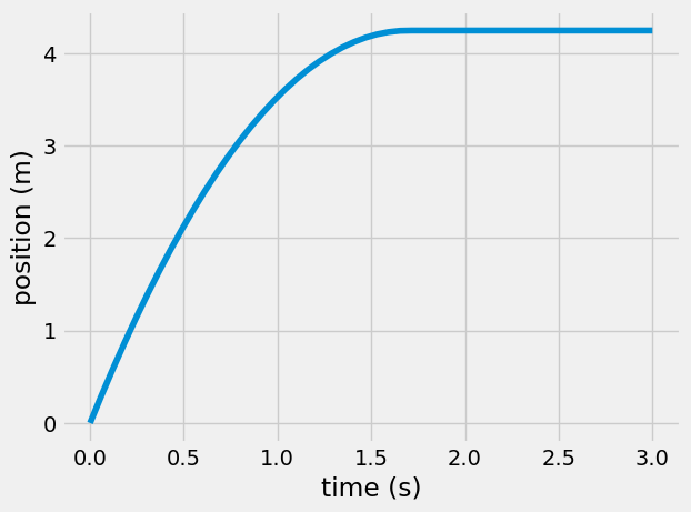
Coulomb friction on a sliding block

This first example, has a small trick. The acceleration is constant, \(-\mu g\), until the velocity is zero. At this point, the block stops moving. To solve for \(x(t)\)

• calculate \(x(t)\) and \(v(t)\) if acceleration is constant

• set the values of \(v(t)<0\) to 0

• set the values of \(x(t)\) given \(v(t)=0\) as the maximum \(x\)

Here, \(\mu=0.3\) and m = 0.5 kg

t = np.linspace(0, 3)
xa = 5*t - 0.5*0.3*9.81*t**2
va = 5 - 0.3*1*9.81*t
va[va < 0] = 0
xa[va == 0] = xa.max()
plt.plot(t, xa)
plt.xlabel('time (s)')
plt.ylabel('position (m)')

Text(0, 0.5, 'position (m)')

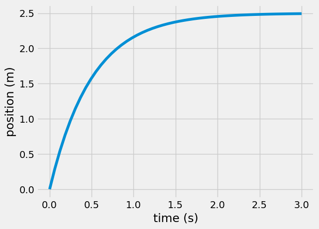
Viscous friction

This second example has a exponentially decaying speed. This type of motion is common in door dampers and shock absorbers. The faster the object moves, the faster it decelerates.

• \(v(t) = v_0 e^{-\frac{b}{m}t}\)

• \(x(t) = \frac{v_0 m}{b}\left(1 - e^{-\frac{b}{m} t}\right)\)

Here, b = 1 kg/s and m = 0.5 kg

m = 0.5
b = 1
xb = 5*m/b*(1-np.exp(-b/m*t))
plt.plot(t, xb)
plt.xlabel('time (s)')
plt.ylabel('position (m)')

Text(0, 0.5, 'position (m)')

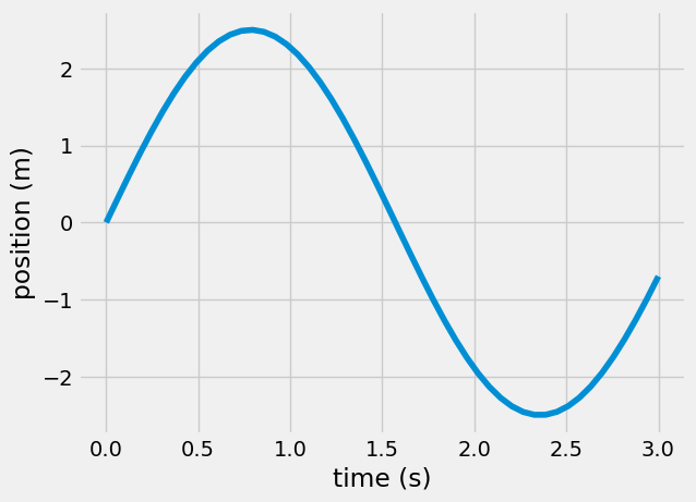
Linear spring and the harmonic oscillator

This third example is a harmonic oscillator. Any object that has a restoring force e.g. a spring attached to a mass, a pendulum swinging, object hanging from a rubber band. The harmonic oscillator is described by the general equation

\(\ddot{x} = -\omega^2 x\)

where \(\omega = \sqrt{\frac{k}{m}}\) for a spring mass. Here, \(k=2~N/m\) and m=0.5 kg.

w = np.sqrt(2/0.5)
xc = 5/w*np.sin(w*t)
plt.plot(t, xc)
plt.xlabel('time (s)')
plt.ylabel('position (m)');

Wrapping up - comparing all three examples

You have plotted three solutions

1. sliding with friction

2. viscous friction

3. harmonic oscillator

Now, you can plot all three together.

plt.plot(t, xa, label = 'friction')
plt.plot(t, xb, label = 'viscous') 
plt.plot(t, xc, label = 'harmonic')
plt.legend();
plt.xlabel('time (s)')
plt.ylabel('position (m)');

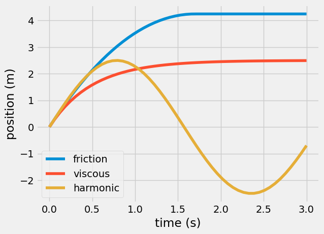
Some similiraties between the three plots

• each plot begins at 0 m

• each plot has the same initial slope

Some differences between the three plots

• the friction and viscous friction have a final position, but the harmonic plot continues to move

• the blue friction plot has two distinct functions: \(\propto t^2\) and \(\propto constant\), but the other plots are continuous functions