import numpy as np
import matplotlib.pyplot as plt
plt.style.use('fivethirtyeight')
plt.rcParams.update({
    "text.usetex": True,
    "font.family": "sans-serif"
})
#plt.rcParams['text.latex.preamble']=[r'sansmath']

from IPython.display import YouTubeVideo
YouTubeVideo('uOq4AbvWF08')

Rolling on hemisphere

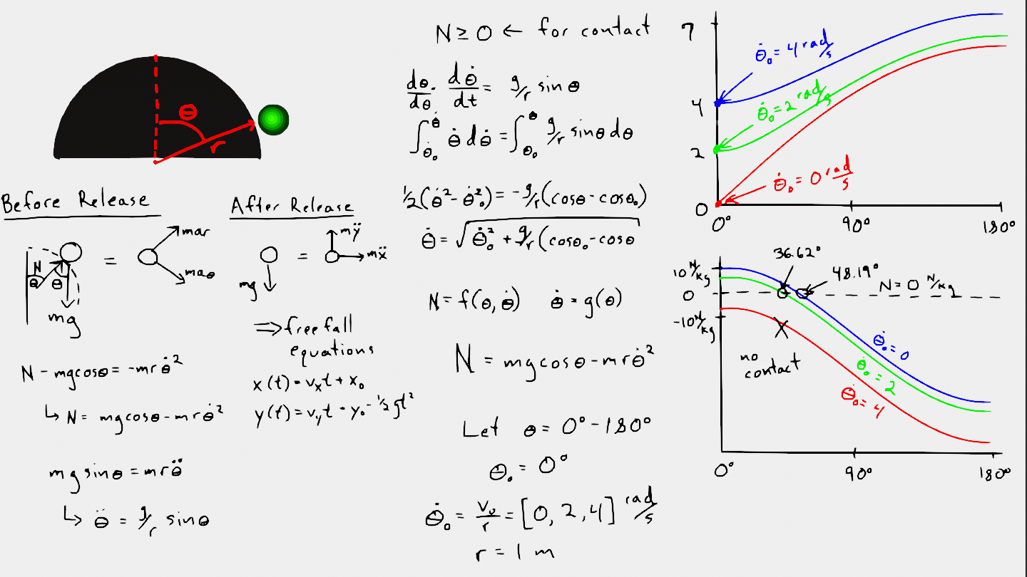
In this example, a small ball with negligible moment of inertia rolls on a hemisphere and loses contact at some point. Your goal is to determine the point where the ball loses contact with the hemisphere. The hemisphere has radius, \(R=1~m\), and the ball has mass \(m=1~kg\).

There are two states in this problem:

1. Ball and hemisphere are in contact with normal force \(N>0\)

2. Ball and hemisphere are not in contact, so normal force \(N=0\)

There cannot be a state where \(N<0\) because that would mean there is an attractive force between the ball and hemisphere.

Equation of motion and contact force

Using the free body diagram and kinetic diagram, you can derive these two equations for state 1 (contact):

1. \(\ddot{\theta} = \frac{g}{R}\sin\theta\)

2. \(N = mg\cos\theta-mR\dot{\theta}^2\)

Integrate equation 1 by using the chain rule,

\(\frac{d\theta}{d\theta}\frac{d\dot{\theta}}{dt} = \frac{g}{R}\sin\theta\)

\(\frac{d\theta}{dt}\frac{d\dot{\theta}}{d\theta} = \frac{g}{R}\sin\theta\)

\(\int_{\dot{\theta}_0}^{\dot{\theta}}\dot{\theta}d\dot{\theta} = \int_{\theta_0}^{\theta}\frac{2g}{R}\sin\theta\)

\(\dot{\theta} = \sqrt{\dot{\theta}_0^2+\frac{g}{R}(\cos\theta_0-\cos\theta)}\)

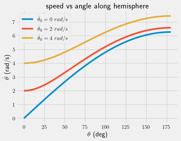
Now, you plot the relation between \(\theta\) and \(\dot{\theta}\) for initial conditions,

• \(\theta_0 = 0~rad\) and \(\dot{\theta}_0=0~rad/s\)

• \(\theta_0 = 0~rad\) and \(\dot{\theta}_0=2~rad/s\)

• \(\theta_0 = 0~rad\) and \(\dot{\theta}_0=4~rad/s\)

__Reflection:__When do you expect the ball to lose contact for 0, 2, and 4 rad/s angular velocities? Will it happen sooner or later if the ball is travelling faster at the top of the hemisphere?

theta = np.linspace(0,np.pi)
dtheta = lambda dt0,theta: np.sqrt(dt0**2+2*9.81/1*(1-np.cos(theta)))
plt.plot(theta*180/np.pi, dtheta(0, theta), label=r'$\dot{\theta}_0=0~rad/s$')
plt.plot(theta*180/np.pi, dtheta(2, theta), label=r'$\dot{\theta}_0=2~rad/s$')
plt.plot(theta*180/np.pi, dtheta(4, theta), label=r'$\dot{\theta}_0=4~rad/s$')
plt.title('speed vs angle along hemisphere')
plt.legend()
plt.xlabel(r'$\theta$ (deg)')
plt.ylabel(r'$\dot{\theta}$ (rad/s)');

Normal force prediction

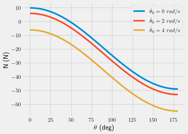
The second equation relates the normal force, \(N\) to \(\theta\) and \(\dot{\theta}\). Now, plot the \(N-vs-\theta\).

\(N = mg\cos\theta-mR\dot{\theta}^2\)

If this equation predicts \(N<0\), then the ball has lost contact with the hemisphere. It will transition into a freefalling object with initial position and velocity,

When N=0, transition state:

• \(\mathbf{r} = R\hat{e}_r=R(\sin\theta\hat{i}+\cos\theta\hat{j})\)

• \(\mathbf{v} = R\dot{\theta}\hat{e}_{\theta}= R\dot{\theta}(\cos\theta\hat{i}-\sin\theta\hat{j})\)

Below, you see the plots for \(N-vs-\theta\) for \(\theta = 0-180^o\),

N0 = 9.81*np.cos(theta)-1*dtheta(0, theta)**2
N2 = 9.81*np.cos(theta)-1*dtheta(2, theta)**2
N4 = 9.81*np.cos(theta)-1*dtheta(4, theta)**2

plt.plot(theta*180/np.pi, N0, label=r'$\dot{\theta}_0=0~rad/s$')
plt.plot(theta*180/np.pi, N2, label=r'$\dot{\theta}_0=2~rad/s$')
plt.plot(theta*180/np.pi, N4, label=r'$\dot{\theta}_0=4~rad/s$')
plt.xlabel(r'$\theta$ (deg)')
plt.ylabel(r'N (N)')
plt.legend()

<matplotlib.legend.Legend at 0x7db3f836f370>

Solving for loss-of-contact

The graph above reveals that at \(\dot{\theta}_0=4~rad/s\), the ball never makes contact with the hemisphere. It skims the top, and falls as

• \(x(t) = 4t~[m]\)

• \(y(t) = 1-\frac{g}{2}t^2~[m]\)

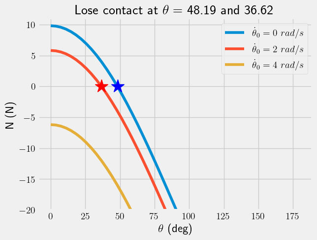
In the cases of \(\dot{\theta}_0=0~and~2~rad/s\), the ball loses contact between \(\theta=25^o-50^o\). You can use algebra to solve for \(N(\theta^*)=0\), where \(\theta^*\) is the location where contact is lost.

or

You have Python here that can solve nolinear problems. Import fsolve from the scipy.optimize library.

from scipy.optimize import fsolve

Defining and solving a nonlinear equation

You have two equations,

1. \(\dot{\theta} = \sqrt{\dot{\theta}_0^2+\frac{g}{R}(\cos\theta_0-\cos\theta)} = g(\dot{\theta}_0,~\theta)\)

2. \(N = mg\cos\theta-mR\dot{\theta}^2 = f(\theta,~\dot{\theta}) = f(\theta, g(\dot{\theta}_0,~\theta))\)

For clarity, you can define equation (1) first, then use it in equation (2) as such

dtheta = lambda dt0,theta: np.sqrt(dt0**2+2*9.81/1*(1-np.cos(theta)))
N = lambda dt0, theta: 9.81*np.cos(theta)-1*dtheta(dt0, theta)**2

thetastar_0 = fsolve(lambda x: N(0, x), np.pi/3)*180/np.pi
thetastar_2 = fsolve(lambda x: N(2, x), np.pi/3)*180/np.pi

plt.plot(theta*180/np.pi, N0, label=r'$\dot{\theta}_0=0~rad/s$')
plt.plot(theta*180/np.pi, N2, label=r'$\dot{\theta}_0=2~rad/s$')
plt.plot(theta*180/np.pi, N4, label=r'$\dot{\theta}_0=4~rad/s$')
plt.plot(thetastar_0[0], N(0,thetastar_0*np.pi/180), 'b*', markersize=20)
plt.plot(thetastar_2[0], N(2,thetastar_2*np.pi/180), 'r*', markersize=20)
plt.xlabel(r'$\theta$ (deg)')
plt.ylabel(r'N (N)')
plt.title(r'Lose contact at $\theta=$ '+'{:.2f} and {:.2f}'.format(thetastar_0[0], thetastar_2[0]))
plt.ylim(-20,11)
plt.legend()

<matplotlib.legend.Legend at 0x7db3ec1c57e0>

Wrapping up

In this notebook, you compared two possible states for a ball rolling on a hemisphere: contact and no contact. You used free body diagrams, kinetic diagrams, and the chain rule to find the transition between contact and no contact.

You used scipy.optimize.fsolve to solve for when a function is 0.