Show code cell source

Hide code cell source

import numpy as np
import matplotlib.pyplot as plt
from scipy.optimize import fsolve
plt.style.use('fivethirtyeight')

Show code cell source

Hide code cell source

from IPython.lib.display import YouTubeVideo
YouTubeVideo('NDZkuxp5n9A')

Pendulum plotting solution

A pendulum is another harmonic oscillator, but you have to linearize the equation of motion. The simple pendulum equation of motion is as such

\(\ddot{\theta} = -\frac{g}{L}\sin\theta\)

where \(g\) is acceleration due to gravity and \(L\) is the length of the pendulum.

Linearize equation of motion

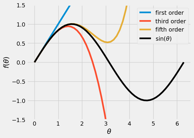
You can’t integrate this equation of motion, so you can take a Taylor series expansion

\(\sin\theta = \theta - \frac{\theta^3}{3!} + \frac{\theta^5}{5!} + ...\)

Now, you can use the first term in the series to create the harmonic oscillator equation

\(\ddot{\theta} = -\omega^2 \theta = -\frac{g}{L} \theta\)

where \(\omega = \sqrt{\frac{g}{L}}\).

You can see how these Taylor series terms diverge from the actual \(\sin\) function below.

Show code cell source

Hide code cell source

theta = np.linspace(0, 2*np.pi)
order1 = theta
order3 = order1 - theta**3/3/2/1
order5 = order3 + theta**5/5/4/3/2/1

plt.plot(theta, order1, label = 'first order')
plt.plot(theta, order3, label = 'third order')
plt.plot(theta, order5, label = 'fifth order')
plt.plot(theta, np.sin(theta), 'k', label = r'$\sin(\theta)$')
plt.ylim((-1.5, 1.5))
plt.legend()
plt.xlabel(r'$\theta$')
plt.ylabel(r'$f(\theta)$');

Plot the solution for the linearized simple pendulum

The solution to the harmonic oscillator is given as such

\(\theta(t) = \theta_0 \cos\omega t + \frac{\dot{\theta}_0}{\omega}\sin\omega t\)

where \(\theta_0\) is the initial angle of the pendulum and \(\dot{\theta}_0\) is the initial angular velocity of the pendulum (+ counter-clockwise/ - clockwise motion).

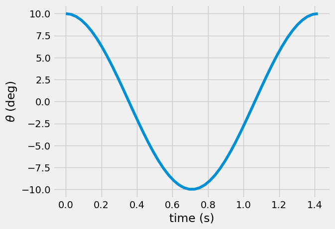
Below, you plot the solution for 1 period of motion for a L = 0.5-m pendulum released from rest at \(\theta_0 = 10^o = \frac{\pi}{18}~rad\).

Note: the time period, \(T=\frac{2\pi}{\omega}~s\) is the time for to move right-to-left, then left-to-right, to its initial position.

L = 0.5 # m
w = np.sqrt(9.81/L)
t = np.linspace(0, 2*np.pi/w)
theta = np.pi/18*np.cos(w*t)
plt.plot(t, theta*180/np.pi)
plt.xlabel('time (s)')
plt.ylabel(r'$\theta$ (deg)')

Text(0, 0.5, '$\\theta$ (deg)')

Motion of the pendulum

The solution plotted above is the orientation of the pendulum. The position of the mass is

\(\mathbf{r} = L\hat{e}_r = L(\sin\theta \hat{i} - \cos\theta \hat{j})\)

where \(\theta = \theta(t)\) that you created above. Below, you plot the x- and y- positions of the simple pendulum.

r = L*np.vstack([np.sin(theta), -np.cos(theta)])

plt.plot(t, r[0,:], label = 'x-location')
plt.plot(t, r[1,:], label = 'y-location')
plt.xlabel('time (s)')
plt.ylabel('position (m)')

Text(0, 0.5, 'position (m)')

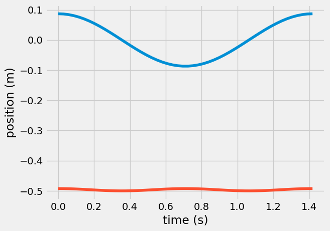
Note: Notice how the x-position has a similar shape to the solution for \(\theta(t)\), but the y-position has very little variation. The angle \(\theta\) is small, \(\theta<<1\), so you can approximate the position as

\(\mathbf{r} = L(\sin\theta \hat{i} - \cos\theta \hat{j}) \approx L\theta\hat{i} - L\hat{j}\)

because the Taylor series expansion for \(\cos(\theta)\) is

\(\cos\theta = 1 - \frac{x^2}{2!} + \frac{x^4}{4!} + ...\)

so you can approximate \(\cos\theta \approx 1\).

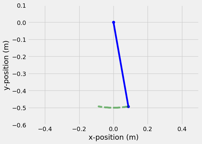
Animation of the pendulum motion

Here, you can see how the pendulum swings. It starts at \(\theta_0=10^o\) and swings left to \(\theta(t=T/2)=-10^o\). In this simple pendulum model, you did not include any effects of air resistance, friction, or damping so the motion will continue to oscillate until acted upon by another system.

Show code cell source

Hide code cell source

fig, ax = plt.subplots()

ax.set_xlim(( -0.5, 0.5))
ax.set_ylim((-0.6, 0.1))
ax.set_xlabel('x-position (m)')
ax.set_ylabel('y-position (m)')

line1, = ax.plot([], [],'bo-')
ax.plot(r[0,:],r[1,:],'g--', alpha=0.5)

from matplotlib import animation
from IPython.display import HTML

def init():
    line1.set_data([], [])
    return (line1, )

def animate(i):
    '''function that updates the line and marker data
    arguments:
    ----------
    i: index of timestep
    outputs:
    --------
    line: the line object plotted in the above ax.plot(...)
    '''
    line1.set_data([0, r[0, i]], [0, r[1, i]])
    return (line1, )

anim = animation.FuncAnimation(fig, animate, init_func=init,
                               frames=range(0,len(t)), interval=50, 
                               blit=True)

HTML(anim.to_html5_video())

---------------------------------------------------------------------------
RuntimeError                              Traceback (most recent call last)
Cell In[6], line 34
     28     return (line1, )
     30 anim = animation.FuncAnimation(fig, animate, init_func=init,
     31                                frames=range(0,len(t)), interval=50, 
     32                                blit=True)
---> 34 HTML(anim.to_html5_video())

File /opt/hostedtoolcache/Python/3.9.23/x64/lib/python3.9/site-packages/matplotlib/animation.py:1265, in Animation.to_html5_video(self, embed_limit)
   1262 path = Path(tmpdir, "temp.m4v")
   1263 # We create a writer manually so that we can get the
   1264 # appropriate size for the tag
-> 1265 Writer = writers[mpl.rcParams['animation.writer']]
   1266 writer = Writer(codec='h264',
   1267                 bitrate=mpl.rcParams['animation.bitrate'],
   1268                 fps=1000. / self._interval)
   1269 self.save(str(path), writer=writer)

File /opt/hostedtoolcache/Python/3.9.23/x64/lib/python3.9/site-packages/matplotlib/animation.py:128, in MovieWriterRegistry.__getitem__(self, name)
    126 if self.is_available(name):
    127     return self._registered[name]
--> 128 raise RuntimeError(f"Requested MovieWriter ({name}) not available")

RuntimeError: Requested MovieWriter (ffmpeg) not available

Wrapping up

In this notebook, you plotted the solution for a simple pendulum and used the kinematic definitions to plot the motion of the pendulum.