Driving forces for moving systems#
In this case study, you want to accelerate a 0.1-kg flywheel with a piston. The desired acceleration of the flywheel is \(\alpha=50~rad/s^2.\) The piston is attached to the link and creates a horizontal driving force. This example demonstrates how we can describe constraints in mathematical forms.
We have two moving bodies:
a flywheel with radius \(r=0.2~m\) and mass \(m=0.1~kg\)
a massless connecting link
Both objects move in a horizontal plane, so their positions have two degrees of freedom to describe position and one degree of freedom that describes orientation.
\(DOF = 3 + 3 = 6\)
Describing constraints#
There are six degrees of freedom for a flywheel and a link, but there are 6 constraints on the system’s motion:
the flywheel is pinned to the ground in the x-dir
the flywheel is pinned to the ground in the y-dir
the top of the link is pinned to the flywheel
the top of the link is pinned to the flywheel
the bottom of the link slides along the horizontal line
the angle of the flywheel has acceleration, \(\alpha=50~rad/s^2\)
\(system~DOF = 6 - 6 = 0~DOF\)
Note: In general, a pin in a planar system creates 2 constraints on motion.
You should recognize at this point that there are 0 differential equations to solve. Once you have calculated the kinematics based upon the system constraints, you can plug in the values and solve for force of the piston. So, start with the kinematic description of motion.
\(\mathbf{r}_2 =\mathbf{r}_{2/3} + \mathbf{r}_3\)
\(r(\sin\theta\hat{i} - \cos\theta \hat{j}) = -L(\cos\theta_{L}\hat{i}-\sin\theta_L\hat{j}) + d\hat{i}\)
this description creates two independent equations
\(-r\sin\theta = -L\cos\theta_{L}+ d\)
\(r\cos\theta = -L\sin\theta_L\)
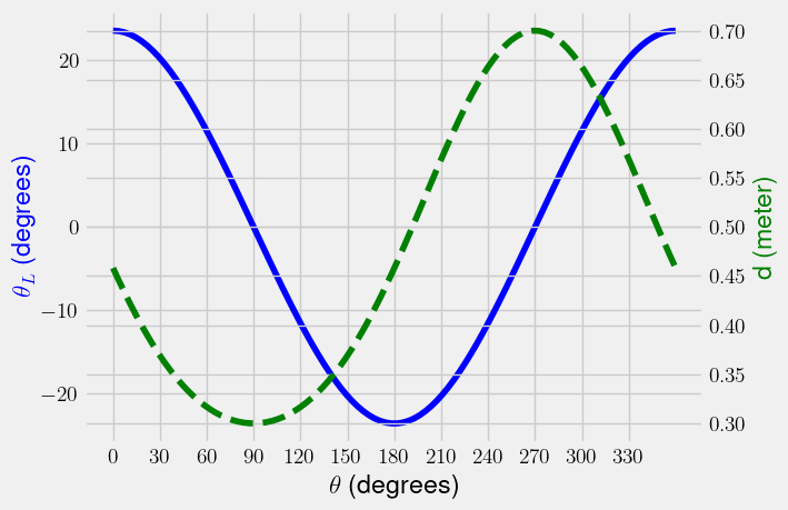
The constraint on \(\theta\) says that \(\theta(t)=\frac{\alpha t^2}{2}\). You need to solve for \(\theta_L\) and \(d\) to determine the full state of the system.
\(\theta_L = \sin^{-1}\left(\frac{r}{L}\cos\theta\right)\)
\(d = L\cos\theta_{L}-r\sin\theta\)

Exercise:#
What is the angular velocity and angular acceleration of the link? \(\dot{\theta}_L\) and \(\ddot{\theta}_L\)
Now, we have solved all of the kinematics we need to solve for the applied piston force. Sometimes, you can look at the Newton-Euler equations for the syatem as a whole, but here we need to separate each component and sum forces and moments.
Flywheel:
\(\sum\mathbf{F}=\mathbf{0}\)
\(\sum M_G = I \alpha\)
Note: If a body is moving, you either have to sum moments about a fixed point or its center of mass. Otherwise, the description of angular acceleration is more involved.
Link:
\(\sum\mathbf{F}=\mathbf{0}\)
\(\sum M = 0\)
Note: when links, cables, or pulleys are assumed to be massless they still obey Newtonian mechanics, but momentum is always zero. So the sum of forces or moments is equal to 0.
The three kinetic equations for the wheel are as such,
\(\sum \mathbf{F}\cdot\hat{i} = F_{2x}+F_{1x} = 0\)
\(\sum \mathbf{F}\cdot\hat{j} = F_{2y}+F_{1y} = 0\)
\(\sum M_{1} = r\hat{e}_r \times (F_{2x}\hat{i}+F_{2y}\hat{j}) = \frac{mr^2}{2}\alpha\)
and the three kinetic equations for the link are as such,
\(\sum \mathbf{F}\cdot\hat{i} = R-F_{2x} = 0\)
\(\sum \mathbf{F}\cdot\hat{j} = -F_{2y} - F_{piston} = 0\)
\(\sum M_{2} = L\hat{b}_1 \times (-F_{piston}\hat{i} + R\hat{j}) = 0\)
The third equation for the link is rearranged to solve for \(R = F\tan\theta_L\). The third equation for the flywheel is rearranged to solve for \(F\) as such
\(rF\cos\theta -rF\tan\theta_L\sin\theta = \frac{mr^2}{2}\alpha\)
finally arriving at
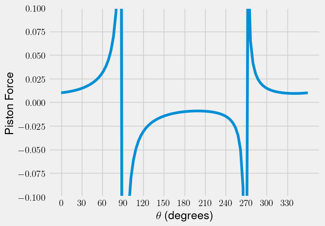
\(F = \frac{mr\alpha}{2}\left(\cos\theta-\tan\theta_L\sin\theta \right)^{-1}\)
Plotted below as a function of flywheel angle, \(\theta\),


