import numpy as np
import matplotlib.pyplot as plt

plt.style.use('fivethirtyeight')

Introduction to Engineering Dynamics

Newtonian Mechanics

There are three laws that define Newtonian Mechanics:

1. An object at rest will stay at rest and an object in motion will remain in motion unless acted upon by an external force \(\sum\mathbf{F}=\mathbf{0}\) and \(\sum\mathbf{M} = \mathbf{0}\)

2. The change in momentum of a body is proportional to the force applied, \(\sum \mathbf{F} = \frac{d}{dt}\left(m\mathbf{v}\right)\) and \(\sum\mathbf{M} = \frac{d}{dt}\left(\mathbf{h}\right)\)

3. For every applied force, there is an equal and opposite reaction force

import sympy

sympy.var('m, g, P_x, P_y, R_y, W_P, L, x')

Fx = P_x
Fy = P_y + R_y - W_P - m*g
Mz = -L/2*m*g + L*R_y - x*W_P

eqns = sympy.Matrix([Fx, Fy, Mz])
A = sympy.solve((eqns[0], eqns[1], eqns[2]), (P_x, P_y, R_y))
Py_function = sympy.lambdify((x, L, W_P, m, g), A[P_y], 'numpy')
Ry_function = sympy.lambdify((x, L, W_P, m, g), A[R_y], 'numpy')

Bridge example: live load no acceleration

Consider a 50-kg person travelling from the left-to-right edges of the bridge at a constant velocity. The acceleration of the person is 0 and the bridge has 0 acceleration.

• \(v_{person} = 10~\frac{m}{s}\)

• \(x_{person} = \int_0^tv_{person}dt = 10t~m\)

The first law defines the study of static structures and objects that are moving slowly or have negligible momentum, \(m\mathbf{v}\). In order to keep the bridge from moving, the total applied force \(\mathbf{F}\) and moments \(\mathbf{M}\) must be equal to \(\mathbf{0}\).

\(\left[\begin{matrix} \sum F_x\\ \sum F_y\\ \sum M_z \end{matrix}\right] = \left[\begin{matrix} P_{x}\\ P_{y} + R_{y} - W_{P} - g m\\ L R_{y} - \frac{L g m}{2} - W_{P} x \end{matrix}\right] = \left[\begin{matrix} 0\\ 0\\ 0\\ \end{matrix}\right]\)

Note: If you set up the equations by separating the unknown variables, \([P_x,~P_y,~R_y]\), from the known variables, you can set up a linear algebra problem. For more information, check out the excellent video series 3Blue 1Brown - Essence of Linear Algebra

\(\left[\begin{matrix} ~1 & 0 & 0\\ 0 & 1 & 1 \\ 0 & 0 &L \end{matrix}\right] \left[\begin{array} ~P_x\\ P_y\\ R_y\end{array}\right]= \left[\begin{matrix} 0\\ W_{P} + mg \\ \frac{mgL}{2}+W_Px\\ \end{matrix}\right]\)

Solving for the reaction forces, you have three equations,

1. \(P_x = 0\)

2. \(P_y = W_P +mg - \frac{mg}{2}-W_P\frac{x}{L}\)

3. \(R_y = \frac{mg}{2}+W_P\frac{x}{L}\)

g = 9.81
L = 10
m = 100
Wp = 50*g

Px = lambda x: 0*x
Py = lambda x: Wp + m*g/2 - Wp*x/L
Ry = lambda x: m*g/2 +Wp*x/L

t = np.linspace(0, 1)
v = 10
x = v*t


plt.plot(x, Px(x), label = r'$P_x$')
plt.plot(x, Py(x), label = r'$P_y$')
plt.plot(x, Ry(x), label = r'$R_y$')
plt.legend()
plt.xlabel('walker position (m)')
plt.ylabel('reaction force (N)')

Text(0, 0.5, 'reaction force (N)')

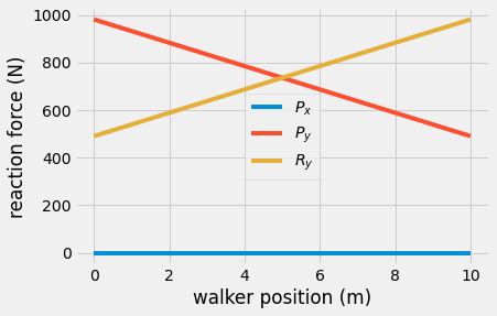
Here you can see the reaction forces at each end of the bridge as a function of the person moving from left, \(x=0~m\) to right, \(x=10~m\). The reaction force increases as the walker moves away from the support.

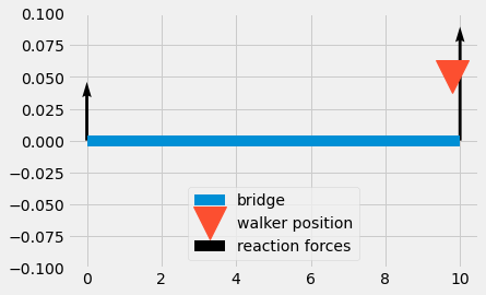
You can watch the reaction forces change in the animation below.

from matplotlib import animation
from IPython.display import HTML
fig, ax = plt.subplots(1,1);
ax.plot(x, x*0, '-', linewidth = 10, label = 'bridge')
Q = ax.quiver([0, 10], 
           [0, 0], 
           [0, 0],
           [Py(x[1]), Ry(x[1])], 
          scale = 3500, label = 'reaction forces')
mark, = ax.plot(x[1], 0.01, 'v', markersize = 30, label = 'walker position')

ax.legend(loc = 'lower center')
ax.set_xlim(-0.5, 10.5)
ax.set_ylim(-0.1, 0.1)

def animate(i):
    """updates the horizontal and vertical vector components by a
    fixed increment on each frame
    """
    Q.set_UVC(np.array([0,  0]), 
              np.array([Py(x[i]), Ry(x[i])]))

    mark.set_data(x[i], 0.05)

    return Q, mark

# you need to set blit=False, or the first set of arrows never gets
# cleared on subsequent frames
anim = animation.FuncAnimation(fig, animate,
                               frames = range(len(t)-1), blit=False)
HTML(anim.to_html5_video())

---------------------------------------------------------------------------
RuntimeError                              Traceback (most recent call last)
Cell In[5], line 31
     27 # you need to set blit=False, or the first set of arrows never gets
     28 # cleared on subsequent frames
     29 anim = animation.FuncAnimation(fig, animate,
     30                                frames = range(len(t)-1), blit=False)
---> 31 HTML(anim.to_html5_video())

File /opt/hostedtoolcache/Python/3.9.19/x64/lib/python3.9/site-packages/matplotlib/animation.py:1285, in Animation.to_html5_video(self, embed_limit)
   1282 path = Path(tmpdir, "temp.m4v")
   1283 # We create a writer manually so that we can get the
   1284 # appropriate size for the tag
-> 1285 Writer = writers[mpl.rcParams['animation.writer']]
   1286 writer = Writer(codec='h264',
   1287                 bitrate=mpl.rcParams['animation.bitrate'],
   1288                 fps=1000. / self._interval)
   1289 self.save(str(path), writer=writer)

File /opt/hostedtoolcache/Python/3.9.19/x64/lib/python3.9/site-packages/matplotlib/animation.py:148, in MovieWriterRegistry.__getitem__(self, name)
    146 if self.is_available(name):
    147     return self._registered[name]
--> 148 raise RuntimeError(f"Requested MovieWriter ({name}) not available")

RuntimeError: Requested MovieWriter (ffmpeg) not available

/tmp/ipykernel_2325/99178247.py:23: MatplotlibDeprecationWarning: Setting data with a non sequence type is deprecated since 3.7 and will be remove two minor releases later
  mark.set_data(x[i], 0.05)

An example with \(a\neq 0\)

Acceleration of a falling ball \(a\neq 0\)

In the previous bridge example, the person and bridge had 0 acceleration. Consider an falling object. Suppose you want to use video capture of a falling ball to compute the acceleration of gravity.

Watch the video of the ball falling.

from IPython.display import YouTubeVideo
vid = YouTubeVideo("xQ4znShlK5A")
display(vid)

We learn from the video that the marks on the panel are every \(0.25\rm{m}\), and on the website they say that the strobe light flashes at about 15 Hz (that’s 15 times per second). The final image on Flickr notes that the strobe fired 16.8 times per second.

The ball is freefalling, so the acceleration is constant, \(a = g = 9.81~\frac{m}{s^2}\). Its not moving left or right, so you can describe its position and velocity as

• \(x(t) = x_0\)

• \(y(t) = y_0 + \dot{y}_0t +\frac{g}{2}t^2\)

where the initial position is \((x_0,~y_0)\), the initial velocity is \((0,~\dot{y}_0)\), and \(t\) is elapsed time. Take a look at the final frame of the compiled positions below.

reader = imageio.get_reader('https://go.gwu.edu/engcomp3vidmit', format='mp4')
image = reader.get_data(1100)

plt.imshow(image, interpolation='nearest');

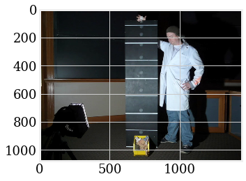
The first position after releasing the ball, is just below the first white line at 125 pixels. The average distance between markers is 495 pixels/meter, so the camera would measure an acceleration

\(g = 9.81~\frac{m}{s^2}\cdot\frac{495~pixels}{1~meter}=4850~\frac{pixels}{s^2}\).

With a little guess-and-check, the initial velocity just below the first white marker is \(\dot{y}_0=800~\frac{pixels}{s}\). The position on the image is then,

\(y(t) = 125 + 800 t + \frac{4850}{2}t^2~pixels\).

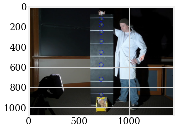
The frames are plotted on top of the image below.

x0 = 720
y0 = 125
bars = np.array([115, 980])
scale = np.diff(bars)/1.75
print(scale, 'px/m')

g = 9.81*scale # m/s^2*d*0.25 px/m = px/s^2


t = np.arange(0, 8, 1)*1/16.8
x = np.ones(len(t))*x0
y = y0 + 800*t + g*t**2/2
plt.clf()
plt.imshow(image)
plt.scatter(x, y, s = 80, facecolor='none', edgecolors='b')

[494.28571429] px/m

<matplotlib.collections.PathCollection at 0x7f993dbd3bb0>

Wrapping up

In this notebook, you looked at two situations

1. forces and motion when acceleration is 0

2. motion when acceleration is \(a\neq0\)

Next, you will define properties of kinetics (forces, energy, and impulse) and kinematics (motion described by position, velocity, acceleration).