Show code cell content Hide code cell content

import numpy as np
import matplotlib.pyplot as plt
from scipy.optimize import fsolve
plt.style.use('fivethirtyeight')

Happy Valentine’s Linkage

In this notebook, you step through the process of defining the kinematics of a four-bar linkage that can draw a heart. Kinematics is the study of the geometry of motion. In this notebook, you predict and draw the geometry of three moving links. To create this solution you will:

• solve a series of nonlinear equations using fsolve

• use solutions to create 2D arrays that vary in time and location

• plot and animate the motion of the four-bar linkage

When you accomplish these steps you will learn:

• How to set up and solve nonlinear equations

• How to describe position and orientation

• How to use NumPy, Scipy, and Matplotlib to create HTML animations

• Why four-bar linkages are so cool

Background

The four-bar linkages consist of 3 moving parts connected to a stationary support. Depending upon the desired output motion, you can vary the lengths of each moving arm, \(l_1,~l_2,~and,l_3\), and the support locations, \(d_x~and~d_y\). A four-bar linkage is an amazing 1-degree-of-freedom system. If one angle is fixed, all of the positions and angles have to be fixed too. Using some trigonometry, you can arrive at these two constraint equations that relate \(\theta_1,~\theta_2,~and~\theta_3\):

1. \(l_1\sin\theta_1+l_2\sin\theta_2-l_3\sin\theta_3 -d_y = 0\)

2. \(l_1\cos\theta_1+l_2\cos\theta_2-l_3\cos\theta_3 -d_x = 0\)

If you have one of the angles, e.g. \(\theta_1\), you use equations 1 and 2 to solve for the other two angles, \(\theta_2~and\theta_3\). Here you can create a function and use fsolve. The function input is a vector with two values and the output is a vector with two values.

\(\bar{f}(\bar{x})= \left[\begin{array}{c} f_1(\theta_2,~\theta_3) \\ f_2(\theta_2,~\theta_3)\end{array}\right]=\left[\begin{array}{c} l_1\sin\theta_1+l_2\sin\theta_2-l_3\sin\theta_3 -d_y\\ l_1\cos\theta_1+l_2\cos\theta_2-l_3\cos\theta_3 -d_x \end{array}\right]\)

Defining your system

The heart-drawing linkage system has the following properties:

• link 1: \(l_1 = 1~m\)

• link 2: \(l_2 = 1~m\)

• link 3: \(l_3 = 1~m\)

• support: \(d_x=0.95~m~and~d_y=0~m\)

The constraint function is defined below as Fbar, a function of \(\theta_1\) and an array of \([\theta_2,~\theta_3]\) as such,

l1 = 1
l2 = 1
l3 = 1
a1 = np.pi/2
dy = 0
dx = 0.95
Fbar = lambda a1,x: np.array([l1*np.sin(a1)+l2*np.sin(x[0])-l3*np.sin(x[1])-dy,
                           l1*np.cos(a1)+l2*np.cos(x[0])-l3*np.cos(x[1])-dx])

Solve for one configuration

Now, solve Fbar using scipy.optimize.fsolve. The inputs are a function, Fbar, and an initial guess, x0. You have to use lambda again to set the angle \(\theta_1\) as a1 = np.pi/2

a1 = np.pi/2
x0 = np.array([0,np.pi/2])
xsol = fsolve(lambda x: Fbar(a1, x), x0)

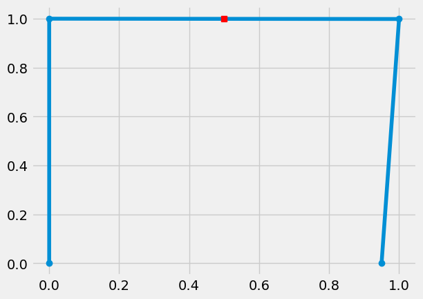
The configuration for \(\theta_1=\frac{\pi}{2}\) is now saved in xsol. To look at the system in this state, define the positions of each hinge and the center of link 2 as such,

x- and y-locations of hinges:

• \(rx = \left[\begin{array}~0\\l_1\cos(\theta_1)\\l_1\cos(\theta_1)+l_2\cos(\theta_2)\\ l_1\cos(\theta_1) + l_2\cos(\theta_2)-l_3\cos(\theta_3)\end{array}\right]\)

• \(ry = \left[\begin{array}~0\\l_1\sin(\theta_1)\\l_1\sin(\theta_1)+l_2\sin(\theta_2)\\ l_1\sin(\theta_1)+l_2\sin(\theta_2)-l_3\sin(\theta_3)\end{array}\right]\)

x- and y-location of point P:

• \(rx = \left[\begin{array}~l_1\cos(\theta_1)+l_2\cos(\theta_2)\end{array}\right]\)

• \(ry = \left[\begin{array}~l_1\sin(\theta_1)+l_2\sin(\theta_2)\end{array}\right]\)

In the Python cell, you define rx and ry to draw the three moving links and rpx and rpy that define point P as such,

rx = np.array([0,
               l1*np.cos(a1),
               l1*np.cos(a1)+l2*np.cos(xsol[0]), 
               l1*np.cos(a1)+l2*np.cos(xsol[0])-l3*np.cos(xsol[1])])
ry = np.array([0,
               l1*np.sin(a1),
               l1*np.sin(a1)+l2*np.sin(xsol[0]), 
               l1*np.sin(a1)+l2*np.sin(xsol[0])-l3*np.sin(xsol[1])])
rpx = l1*np.cos(a1)+l2/2*np.cos(xsol[0])
rpy = l1*np.sin(a1)+l2/2*np.sin(xsol[0])

plt.plot(rx,ry,'o-')
plt.plot(rpx,rpy,'rs')
#plt.axis([-0.5, 1.5, -0.6, 0.6])

[<matplotlib.lines.Line2D at 0x7f8e9ca1d0a0>]

Solve for the whole cycle

You have verified the solution works for one angle, a1. Now, you can create an array of a1 and solve for the angles at each configuration as you rotate link 1.

1. define a1 as a linspace

2. initialize a2 and a3 as zeros with a1.shape

3. use a for-loop to fsolve each angle a2 and a3 given a1

4. save the values of a2 and a3 in each step

a1 = np.linspace(-np.pi/2,3*np.pi/2,500)
a2 = np.zeros(a1.shape) # initialize
a3 = np.zeros(a1.shape) # initialize
for i, a in enumerate(a1):
    xsol = fsolve(lambda x: Fbar(a,x), xsol) # solve
    a2[i] = xsol[0] # save value for a2
    a3[i] = xsol[1] # save value for a3
    

Verify cycle solution

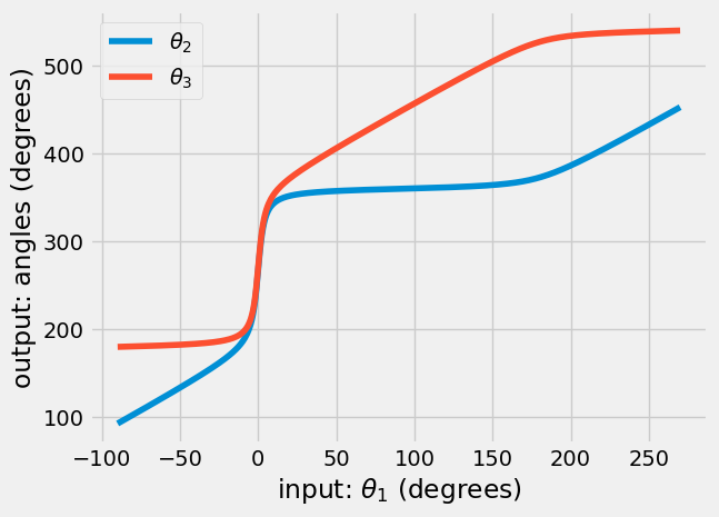
Now, you can see how the functions, \(\theta_2=f_{\theta_2}(\theta_1)\) and \(\theta_3=f_{\theta_3}(\theta_1)\). This is another verification step, to see if there are any discontinuities in the solution that could cause problems.

plt.plot(a1*180/np.pi, a2*180/np.pi, label = r'$\theta_2$')
plt.plot(a1*180/np.pi, a3*180/np.pi, label = r'$\theta_3$')
plt.legend()
plt.xlabel(r'input: $\theta_1$ (degrees)')
plt.ylabel('output: angles (degrees)')

Text(0, 0.5, 'output: angles (degrees)')

Time to animate

Now, you are ready to animate. You have the angles for the entire cycle of motion for the four-bar linkage. Now, you need to import matplotlib.animation and IPython.display.HTML.

Import functions

from matplotlib import animation
from IPython.display import HTML

These two functions allow you:

1. create an animation

2. display it in a browser

Define lines and paths

Then, use the solutions for a1, a2, and a3 to plot the hinge locations and point P as such

rx = np.array([np.zeros(a1.shape),
               l1*np.cos(a1),
               l1*np.cos(a1)+l2*np.cos(a2), 
               l1*np.cos(a1)+l2*np.cos(a2)-l3*np.cos(a3)])
ry = np.array([np.zeros(a1.shape),
               l1*np.sin(a1),
               l1*np.sin(a1)+l2*np.sin(a2), 
               l1*np.sin(a1)+l2*np.sin(a2)-l3*np.sin(a3)])

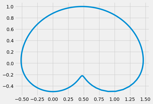
rpx = l1*np.cos(a1)+l2/2*np.cos(a2)
rpy = l1*np.sin(a1)+l2/2*np.sin(a2)

plt.plot(rpx,rpy)

[<matplotlib.lines.Line2D at 0x7f8e9c844520>]

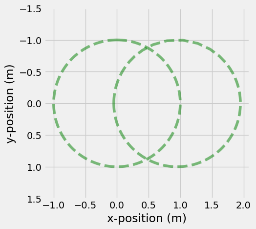
Set up figure and axes

Plotting just the solution for point P’s path, you see the heart shape is upside-down. In the animation, you can reverse the y-axis to flip the drawing. Here, you set up the figure to create the animation:

• ax: axis for plotting the lines

• line1: lines that draw the three moving links rx and ry

• line2: line that updates the heart drawing as links move along paths

fig, ax = plt.subplots()

#ax.set_xlim(( -30, 30))
ax.set_ylim((1.5, -1.5))
ax.set_xlabel('x-position (m)')
ax.set_ylabel('y-position (m)')

line1, = ax.plot([], [],'bo-')
line2, = ax.plot([], [],'r')
ax.plot(rx[1,:],ry[1,:],'g--', alpha=0.5)
ax.plot(rx[2,:],ry[2,:],'g--', alpha=0.5)

[<matplotlib.lines.Line2D at 0x7f8e9c73e460>]

Define initializing and animation functions

Create an initializing (init) function that clears the previous lines

def init():
    line1.set_data([], [])
    line2.set_data([], [])
    return (line1, line2, )

Create an animating (animate) function that updates the lines. The links should be drawn for a given column, i.e. line1 is defined as rx[:, i] and ry[:, i], but you want the path of the heart up to the current frame i.e. line2 is defined as rpx[:i] and rpy[:i].

def animate(i):
    '''function that updates the line and marker data
    arguments:
    ----------
    i: index of timestep
    outputs:
    --------
    line: the line object plotted in the above ax.plot(...)
    '''
    line1.set_data(rx[:, i], ry[:,i])
    line2.set_data(rpx[:i], rpy[:i])
    return (line1, line2 )

Create the animation and display

Create an animation (anim) variable using the animation.FuncAnimation

anim = animation.FuncAnimation(fig, animate, init_func=init,
                               frames=range(0,len(a1)), interval=10, 
                               blit=True)

HTML(anim.to_html5_video())

---------------------------------------------------------------------------
RuntimeError                              Traceback (most recent call last)
Cell In[14], line 1
----> 1 HTML(anim.to_html5_video())

File /opt/hostedtoolcache/Python/3.9.19/x64/lib/python3.9/site-packages/matplotlib/animation.py:1285, in Animation.to_html5_video(self, embed_limit)
   1282 path = Path(tmpdir, "temp.m4v")
   1283 # We create a writer manually so that we can get the
   1284 # appropriate size for the tag
-> 1285 Writer = writers[mpl.rcParams['animation.writer']]
   1286 writer = Writer(codec='h264',
   1287                 bitrate=mpl.rcParams['animation.bitrate'],
   1288                 fps=1000. / self._interval)
   1289 self.save(str(path), writer=writer)

File /opt/hostedtoolcache/Python/3.9.19/x64/lib/python3.9/site-packages/matplotlib/animation.py:148, in MovieWriterRegistry.__getitem__(self, name)
    146 if self.is_available(name):
    147     return self._registered[name]
--> 148 raise RuntimeError(f"Requested MovieWriter ({name}) not available")

RuntimeError: Requested MovieWriter (ffmpeg) not available

Wrapping up

There you have it, a heart-drawing four-bar linkage. This solution required arrays, nonlinear solutions, and some trigonometry to build locations of hinges and links.

Try changing the lengths the different links or changing the fixed positions. What else can you draw?