HW_00 - Interacting with Python and Physics

Content modified under Creative Commons Attribution license CC-BY 4.0, code under BSD 3-Clause License © 2020 R.C. Cooper

These notebooks are a combination of original work and modified notebooks from Engineers Code learning modules. The learning modules are covered under a Creative Commons License, so we can modify and publish and give credit to L.A. Barba and N.C. Clementi.

Our first goal is to interact with Python and handle data in Python. But let’s also learn a little bit of background.

Show code cell content Hide code cell content

import numpy as np
import matplotlib.pyplot as plt
plt.style.use('fivethirtyeight')

What is Python?

Python was born in the late 1980s. Its creator, Guido van Rossum, named it after the British comedy “Monty Python’s Flying Circus.” His goal was to create “an easy and intuitive language just as powerful as major competitors,” producing computer code “that is as understandable as plain English.”

We say that Python is a general-purpose language, which means that you can use it for anything: organizing data, scraping the web, creating websites, analyzing sounds, creating games, and of course engineering computations.

Python is an interpreted language. This means that you can write Python commands and the computer can execute those instructions directly. Other programming languages—like C, C++ and Fortran—require a previous compilation step: translating the commands into machine language. A neat ability of Python is to be used interactively. [Fernando Perez](https://en.wikipedia.org/wiki/Fernando_Pérez_(software_developer) famously created IPython as a side-project during his PhD. The “I” in IPython stands for interactive: a style of computing that is very powerful for developing ideas and solutions incrementally, thinking with the computer as a kind of collaborator.

Why Python?

Because it’s fun! With Python, the more you learn, the more you want to learn. You can find lots of resources online and, since Python is an open-source project, you’ll also find a friendly community of people sharing their knowledge. And it’s free!

Python is known as a high-productivity language. As a programmer, you’ll need less time to develop a solution with Python than with most other languages. This is important to always bring up whenever someone complains that “Python is slow.” Your time is more valuable than a machine’s! (See the Recommended Readings section at the end of this lesson.) And if we really need to speed up our program, we can re-write the slow parts in a compiled language afterwards. Because Python plays well with other languages :–)

The top technology companies use Python: Google, Facebook, Dropbox, Wikipedia, Yahoo!, YouTube… Python took the No. 1 spot in the interactive list of The 2017 Top Programming Languages, by IEEE Spectrum (IEEE is the world’s largest technical professional society).

Python is a versatile language, you can analyze data, build websites (e.g., Instagram, Mozilla, Pinterest), make art or music, etc. Because it is a versatile language, employers love Python: if you know Python they will want to hire you. —Jessica McKellar, ex Director of the Python Software Foundation, in a 2014 tutorial.

Python as a calculator

You can use Python as a calculator. Try using these symbols below to do some math with integers and floating point numbers.

+   -   *   /   **   %   //

The % symbol is the modulo operator (divide and return the remainder), and the double-slash, // is floor division.

2 + 2

4

1.25 + 3.65

4.9

5 - 3

2

2 * 4

8

7 / 2

3.5

7//2

3

2**3

8

Let’s see an interesting case:

9**1/2

4.5

What happened? Isn’t \(9^{1/2} = 3\)? (Raising to the power \(1/2\) is the same as taking the square root.) Did Python get this wrong?

Compare with this:

9**(1/2)

3.0

Yes! The order of operations matters!

If you don’t remember what we are talking about, review the Arithmetics/Order of operations. A frequent situation that exposes this is the following:

3 + 3 / 2

4.5

(3 + 3) / 2

3.0

In the first case, we are adding \(3\) plus the number resulting of the operation \(3/2\). If we want the division to apply to the result of \(3+3\), we need the parentheses.

Exercises:

Use Python (as a calculator) to solve the following two problems:

1. The volume of a sphere with radius \(r\) is \(\frac{4}{3}\pi r^3\). What is the volume of a sphere with diameter 6.65 cm?

   For the value of \(\pi\) use 3.14159 (for now). Compare your answer with the solution up to 4 decimal numbers.

   Hint: 523.5983 is wrong and 615.9184 is also wrong.

2. Suppose the cover price of a book is \(\$ 24.95\), but bookstores get a \(40\%\) discount. Shipping costs \(\$3\) for the first copy and \(75\) cents for each additional copy. What is the total wholesale cost for \(60\) copies? Compare your answer with the solution up to 2 decimal numbers.

To reveal the answers, highlight the following line of text using the mouse:

Answer exercise 1: 153.9796 Answer exercise 2: 945.45

Variables and their type

Variables consist of two parts: a name and a value. When we want to give a variable its name and value, we use the equal sign: name = value. This is called an assignment. The name of the variable goes on the left and the value on the right.

The first thing to get used to is that the equal sign in a variable assignment has a different meaning than it has in Algebra! Think of it as an arrow pointing from name to value.

We have many possibilities for variable names: they can be made up of upper and lowercase letters, underscores and digits… although digits cannot go on the front of the name. For example, valid variable names are:

    x
    x1
    X_2
    name_3
    NameLastname

Keep in mind, there are reserved words that you can’t use; they are the special Python keywords.

OK. Let’s assign some values to variables and do some operations with them:

a = 3 

b = 4.5

Exercise:

Print the values of the variables a and b.

Let’s do some arithmetic operations with our new variables:

a + b

7.5

2**a

8

b - 3

1.5

And now, let’s check the values of x and y. Are they still the same as they were when you assigned them?

print(a)

3

print(b)

4.5

NumPy arrays expand calculations across new dimensions

Consider the case of a projectile motion problem. A ball is thrown from an initial height with an initial x- and y-velocity. Gravity acts along the y-direction and no forces act along the x-direction.

Let’s give the ball some initial parameters,

• \(x_0 = 0~m\)

• \(y_0 = 1.2~m\) someone throwing the ball

• \(v_{x0} = 16~m/s\)

• \(v_{y0} = 16~m/s\)

and our kinematic equations to describe the ball’s position over time are

• \(x(t) = x_0 + v_{x0}t\)

• \(y(t) = y_0 + v_{y0}t - \frac{1}{2}gt^2\)

In this problem, we can use Python to calculate the position at any point in time, but what if we want to know the position for times from 0 to 5 seconds? or we want to solve for when the height is \(0~m\) and it strikes the ground?

This is a time to use NumPy arrays! We can define the independent variable, t, and then calculate the positions, x and y with our equations

x0 = 0 # m
y0 = 1.2 # m
vx = 16 # m/s
vy = 16 # m/s
g = 9.81 # m/s/s

t = np.array([0, 1, 2, 3, 4, 5])

x = x0 + vx*t
y = y0 + vy*t - g/2*t**2

x

array([ 0, 16, 32, 48, 64, 80])

y

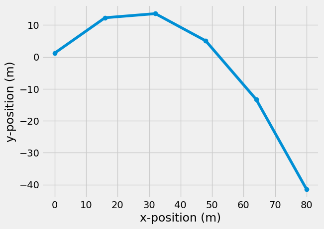
array([  1.2  ,  12.295,  13.58 ,   5.055, -13.28 , -41.425])

Great! Now, we have the position of the ball at different times, but it looks like it hit the ground between 3 and 4 seconds. Let’s plot the path (y-vs-x plot) and see how far the ball travelled.

We’ll use the Matplotlib Pyplot commands to view the equations,

plt.plot(x, y, 'o-')
plt.xlabel('x-position (m)')
plt.ylabel('y-position (m)')

Text(0, 0.5, 'y-position (m)')

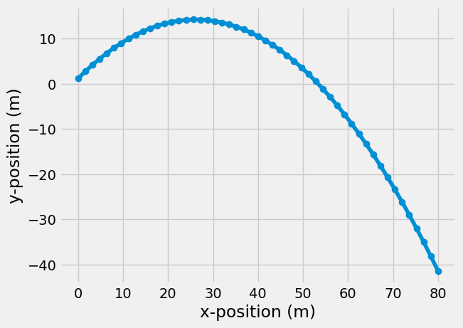
Great start, but we might want more positions during that time, so we can use a built-in function, np.linspace, to define the starting and ending time and increase the number of timesteps,

np.linspace(start, stop, number of steps)

t = np.linspace(0, 5, 51)
x = x0 + vx*t
y = y0 + vy*t - g/2*t**2

plt.plot(x, y, 'o-')
plt.xlabel('x-position (m)')
plt.ylabel('y-position (m)')

Text(0, 0.5, 'y-position (m)')

Even better, but I would like to get rid of the negative values of y-position.

Logical and comparison operators

The Python comparison operators are: <, <=, >, >=, ==, !=. They compare two objects and return either True or False: smaller than, smaller or equal, greater than, greater or equal, equal, not equal. Try it!

c = 3
d = 5

c > d

False

We can assign the truth value of a comparison operation to a new variable name:

z = c > d

z

False

type(z)

bool

Logical operators are the following: and, or, and not. They work just like English (with the added bonus of being always consistent, not like English speakers!). A logical expression with and is True if both operands are true, and one with or is True when either operand is true. And the keyword not always negates the expression that follows.

Let’s do some examples:

e = 5
f = 3
g = 10

e > f and f > g

False

Remember that the logical operator and is True only when both operands are True. In the case above the first operand is True but the second one is False.

If we try the or operation using the same operands we should get a True.

e > f or f > g

True

And the negation of the second operand results in …

not f > g

True

Exercise:

What is happening in the case below? Play around with logical operators and try some examples.

e > f and not f > g

True

Logical operations for Arrays

We can use logical operations to “index” arrays. Indexing an array is a way of choosing subsets of numbers within the array. For example, if our array is

my_array = np.array([0, 1, 2, 3, 4, 5])

we can grab just the even numbers by starting at 0 and going to the end with steps of 2

my_array[0::2]

array([0, 2, 4])

or show all the numbers before 4 with steps of 1

my_array[0:4:1]

array([0, 1, 2, 3])

Now that we can index the array, we could find the negative y-positions indices and plot everything else

or

we could try some Boolean indexing. Consider my_array if I want to see how many values are less than 4

my_array < 4

array([ True,  True,  True,  True, False, False])

The same way we can create array math equations, we can make array Boolean equations. This becomes even more powerful because we can use Boolean arrays to index other arrays,

• True: returns a value

• False: excludes the value

index_less_than_4 = my_array < 4

my_array[index_less_than_4]

array([0, 1, 2, 3])

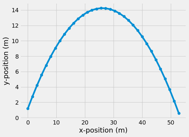
Try this out for our projectile ball, so we can cut out the negative y-values

ground_index = y > 0

plt.plot(x[ground_index], y[ground_index], 'o-')
plt.xlabel('x-position (m)')
plt.ylabel('y-position (m)')

Text(0, 0.5, 'y-position (m)')

We can also grab the last positive y-value using [-1],

print('at time {:1.3f} s, the ball is {:1.2f} m from ground'.format(t[ground_index][-1], y[ground_index][-1]))

at time 3.300 s, the ball is 0.58 m from ground

If we want to get closer to the ground with our calculations, we can increase the number of timesteps in np.linspace e.g. np.linspace(0, 5, 501) will calculate the position every 0.01 s.

What we’ve learned

• Using Python as a calculator.

• Concepts of variable, type, assignment.

• Creating NumPy arrays

• Plotting results with Matplotlib’s Pyplot

• Special variables: True, False, None.

• Indexing NumPy arrays

References

If you want to dig deeper into using Python for engineering and physics, check out these references:

1. Effective Computation in Physics: Field Guide to Research with Python (2015). Anthony Scopatz & Kathryn D. Huff. O’Reilly Media, Inc.

2. Python for Everybody: Exploring Data Using Python 3 (2016). Charles R. Severance. PDF available

3. Think Python: How to Think Like a Computer Scientist (2012). Allen Downey. Green Tea Press. PDF available

Problems

1. Calculate some properties of a rectangular box that is 12.5”\(\times\)11”\(\times\)14” and weighs 31 lbs

a. What is the volume of the box?

b. What is the average density of the box?

c. Its time to ship your box. Check that the dimensions from largest to smallest are

• less than 15”

• less than 13”

• less than 12”

• weight is less than 35 lb

print out a True or False statement for each comparison. Use the and to check that all 4 statements are True.

2. A chair slides across a waxed floor. Your goal is to show how far it moved and where it stopped. The only force slowing the chair down is the force of friction, so the kinematic equations are

• \(x(t) = x_0 + v_0 t - \frac{1}{2}\mu g t^2\)

• \(v(t) = v_0 - \mu g t\)

but, these equations are only valid while \(v(t)>0\)

• \(\mu = 0.1\)

• \(x_0 = 0~m\)

• \(v_0 = 3~m/s\)

• \(g = 9.81~\frac{m}{s^2}\)

a. Plot the position and velocity from 0-5 seconds

b. Update the plot to only show time, position, and velocity while \(v(t)>0\)

c. How far did the chair slide?