import numpy as np
import matplotlib.pyplot as plt
plt.style.use('fivethirtyeight')

Galileo’s rolling experiment

Galileo is credited with creating the field of kinematics. One of his earliest experiments was to measure the position and speed of a ball rolling on an incline plane. He determined that the position was proportional to the square of time. This means that the motion is described by constant acceleration.

Kinematics of rolling

Here, consider a lacrosse ball rolling on a slope. Before you create the equations of motion for the ball, consider the kinematics of a rolling ball. The point-of-contact between the ground and ball has the same velocity both on the ball and the ground. The ground isn’t moving, so the point-of-contact isn’t moving.

In order to move forward, the ball rotates. One rotation is one circumference of the sphere. You can write this as a kinematic constraint as such

\[d = -R\theta\]

where \(d\) is the distance along the slope, \(R=??\) is the radius of the ball, and \(\theta\) is the angle that the ball has rotated counterclockwise thus the negative sign. This constraint equation also relates the speed and acceleration of the ball to its rotation rate as such,

• velocity: \(v=-R\dot{\theta}\)

• acceleration: \(a = -R\ddot{\theta}\).

These are general constraints for an object that rolls without slipping.

Kinetics of rolling

The ball rolls down an incline of 5\(^o\). Start with the free body diagram.

Using the Newton-Euler equations for planar motion, you have three equations,

1. \(mg\sin\alpha - F_f = m\ddot{x}\)

2. \(N-mg\cos\alpha = m\ddot{y}\)

3. \(-R\cdot F_f = I_{zz}\ddot{\theta}\)

where \(\alpha\) is the angle of the plane, \(mg\) is the weight of the ball, \(F_f\) is the force of friction between the ball and the slope, \(N\) is the normal force from the plane, \(\ddot{x}\) is the acceleration along the slope, \(\ddot{y}=0\) is the acceleration normal to the plane which is zero if its rolling, \(I_{zz}=\frac{2}{5}mR^2\) is the moment of inertia for a sphere, and \(\ddot{\theta}\) is the angular acceleration of the ball. These three equations have four unknowns:

Unknown:

• \(F_f\): force of friction

• \(N\): normal force

• \(\ddot{x}\): acceleration

• \(\ddot{\theta}\): angular acceleration

Note: Friction is often introduced as Coulomb’s friction law \(F_f=\mu N\), where \(\mu\) is the coefficient of friction. With rolling objects, the relationship is better represented by an inequality, \(F_f \leq \mu N\). Coulomb friction represents the upper bound on the force of friction, it cannot be universally applied as an equality.

Solving for the motion of the ball on a slope

You now have 1 constraint equation and 3 kinetic equations with four unknowns. You can set up the 4 equations and 4 unknowns

1. \(\ddot{\theta} = \frac{\ddot{x}}{R}\)

2. \(g\sin\alpha - \frac{F_f}{m} = \ddot{x}\)

3. \(\frac{N}{m} = g\cos\alpha\)

4. \(-R\frac{F_f}{m} = -\frac{2}{5}R^2 \frac{\ddot{x}}{R}\)

rearranging for \(\ddot{x}\), you can integrate using initial conditions \(x(0) = \dot{x}(0)=0\),

\[\ddot{x} =\frac{g\sin\alpha}{1+\frac{2}{5}}\]

\[\dot{x}(t) =\frac{g\sin\alpha}{1+\frac{2}{5}}t\]

\[x(t) =\frac{g\sin\alpha}{2(1+\frac{2}{5})}t^2\]

t = np.linspace(0, 1)
a = 9.81*np.sin(5*np.pi/180)/(1+2/5)
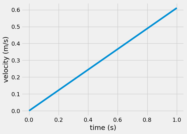
v = a*t
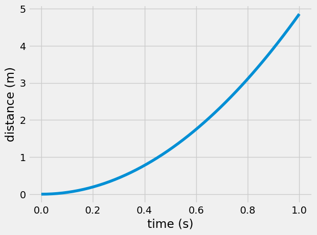
x = a/2*t**2
plt.plot(t, v)
plt.xlabel('time (s)')
plt.ylabel('velocity (m/s)')

Text(0, 0.5, 'velocity (m/s)')

plt.plot(t, x/0.01/np.pi/2)
plt.xlabel('time (s)')
plt.ylabel('distance (m)')

Text(0, 0.5, 'distance (m)')

Wrapping up

In this notebook, you

• defined kinematic constraints for rolling

• used a free body diagram and kinetic diagram to set up 3 planar equations of motion

• integrated the equations of motion to plot the position and rotation of a ball rolling on a plane