Building Quiz_05¶

Swinging pendulum in viscous fluid

A pendulum is placed inside a viscous fluid. The motion of the pendulum is subject to 2 external forces:

gravity: \(F_g = mg\)
viscous damping: \(F_f =-b\mathbf{v}= -bL\dot{\theta}\hat{e}_{\theta}\)

The final equation of motion is as such

\[\ddot{\theta}+\frac{b}{m}\dot{\theta}+\frac{g}{L}\sin\theta = 0\]

a. Find the variation in the Lagrangian, \(\delta L\)

b. Write the nonconservative virtual work, \(\delta W^{NC}\)

c. Show that \(\delta L + \delta W^{NC}=0\) results in the final equation of motion.

Linear solution¶

Equation of motion in a linearized system:

\[\ddot{\theta}+\frac{b}{m}\dot{\theta}+\frac{g}{L}\theta = 0\]

\[\ddot{\theta}+2\zeta\omega\dot{\theta}+\omega^2\theta = 0\]

where

\(\omega = \sqrt{\frac{g}{L}}\)
\(\zeta = \frac{b}{2m}\sqrt{\frac{l}{g}}\)

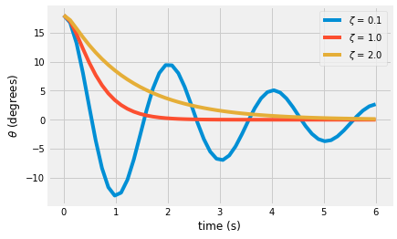
This is a damped harmonic oscillator, so the solution will come in 3 forms:

underdamped \(\zeta<1\)
critically damped \(\zeta = 1\)
overdamped \(\zeta > 1\)

Consider a pendulum with length, \(L=1~m\), mass of \(m=0.1~kg\), and 3 different damping ratios:

\(\zeta\)	b [kg/s]
0.1	0.063
1	0.63
2	1.25

\(\theta(t) = e^{-\zeta\omega t}(a_1 e^{i\omega t\sqrt{1-\zeta^2}} + a_2 e^{-i\omega t\sqrt{1-\zeta^2}})\)

\(\dot{\theta}(t) = -\zeta\omega e^{-\zeta\omega t}(a_1 e^{i\omega t\sqrt{1-\zeta^2}} + a_2 e^{-i\omega t\sqrt{1-\zeta^2}}) +i\omega \sqrt{1-\zeta^2}e^{-\zeta\omega t}(a_1 e^{i\omega t\sqrt{1-\zeta^2}} - a_2 e^{-i\omega t\sqrt{1-\zeta^2}})\)

\[\theta_0 = a_1 +a_2\]

\[\dot{\theta}_0 = -\zeta\omega (a_1 +a_2) +i\omega\sqrt{1-\zeta^2}(a_1-a_2)\]

\[\begin{split}\mathbf{A} \left[\begin{array} ~a_1 \\ a_2 \end{array}\right] = \left[\begin{array} ~\theta_0\\ \dot{\theta}_0\end{array}\right]\end{split}\]

where

\[\begin{split}\mathbf{A} = \left[\begin{array} ~1 & 1 \\ -\zeta\omega +i\omega\sqrt{1-\zeta^2} & -\zeta\omega -i\omega\sqrt{1-\zeta^2} \end{array}\right]\end{split}\]

Note: The default np.sqrt returns an error if you ask for np.sqrt(-1). Above, the numpy.lib.scimath.sqrt is imported to allow complex number algebra as such: from numpy.lib.scimath import sqrt

L = 1
g = 9.81
m = 0.1
z = 0.1
w = sqrt(g/L)
def find_constants(state0, z):
    A = np.array([[1, 1], 
                  [1j*w*sqrt(1-z**2)-z*w, -1j*w*sqrt(1-z**2)-z*w]])
    b = np.array(state0)

    a = np.linalg.solve(A,b)
    return a

theta = lambda t, a, z: np.exp(-w*z*t)*(a[0]*np.exp(1j*w*t*sqrt(1-z**2))+a[1]*np.exp(-1j*w*t*sqrt(1-z**2)))
dtheta = lambda t, a, z: -w*z*np.exp(-w*z*t)*(a[0]*np.exp(1j*w*t*sqrt(1-z**2)) +\
                                              a[1]*np.exp(-1j*w*t*sqrt(1-z**2)))+\
                        1j*w*t*sqrt(1-z**2)*np.exp(-w*z*t)*(a[0]*np.exp(1j*w*t*sqrt(1-z**2)) -\
                                              a[1]*np.exp(-1j*w*t*sqrt(1-z**2)))

t = np.linspace(0,6)
for z in [0.1, 0.9999, 2]:
    a = find_constants([np.pi/10, 0], z)
    plt.plot(t, 180/np.pi*theta(t, a, z).real, label = r'$\zeta$ = {:.1f}'.format(z))
plt.xlabel('time (s)')
plt.ylabel(r'$\theta$ (degrees)')
plt.legend();

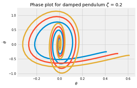
Phase plot for damped system¶

The phase plot for a system plots the input state variables, i.e. \(\theta~and~\dot{\theta}\). In a previous notebook, you looked at the results for an undamped system. With damping, both state variables move towards 0.

z= 0.2 #0.9999
t = np.linspace(0,10, 200)
for pert in [0.1, 0.2, 0.3]:
    a = find_constants([np.pi/10+pert, 0], z)
    plt.plot(theta(t, a, z).real, dtheta(t, a, z).real)

plt.title('Phase plot for damped pendulum $\zeta$ = {:.1f}'.format(z))
plt.xlabel(r'$\theta$')
plt.ylabel(r'$\dot{\theta}$');

Approximate nonlinear solution¶

The final equation of motion is not linear for \(\theta \approx 1\),

\[\ddot{\theta}+\frac{b}{m}\dot{\theta}+\frac{g}{L}\sin\theta = 0.\]

You can numerically integrate this equation for any angle \(\theta\)

create 2 first-order differential equations \(\dot{\mathbf{y}} = f(\mathbf{y})\) where \(\mathbf{y}=[\theta,~\dot{\theta}]\)
use solve_ivp to integrate the equation with initial conditions

def damped_pendulum(t, y, z, w=sqrt(g/L)):
    '''
    damped_pendulum(t, y, z, w)
    
    Return the derivative for a damped pendulum system
    dy[1] + 2*z*w*y[1] + w**2*sin(y[0])
    
    Parameters
    ----------
    t: current time
    y: current state = [theta (rad), dtheta/dt (rad/s)]
    z: damping ratio (determined from eqn of motion)
    w: natural frequency for linear system
    
    Returns
    -------
    dy: derivative of state, y, at time, t 
        [dtheta/ddt (rad/s), ddtheta/ddt (rad/s/s)]

    '''
    dy = np.zeros(y.shape)
    dy[0] = y[1]
    dy[1] = -2*w*z*y[1] - w**2*np.sin(y[0])
    return dy

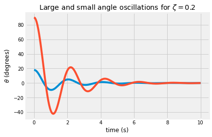
Integrate the exact differential equation with an approximation¶

The differential equation is now exact, but you don’t have a way to solve for the exact function \(\theta(t)\). Use the function solve_ivp to find the solution over a given time interval [0, 10] seconds and evaluated at the same points as the previous linear solution, t_eval = t.

sol = solve_ivp(lambda t, y: damped_pendulum(t, y, 0.2), 
                [0, 10], # timespan [ 0s to 10s]
                [np.pi/10, 0], # initial conditions [18 deg, 0 rad/s]
                t_eval = t)

plt.plot(sol.t, 180/np.pi*sol.y[0])
sol = solve_ivp(lambda t, y: damped_pendulum(t, y, 0.2), 
                [0, 10], # timespan [ 0s to 10s]
                [np.pi/2, 0], # initial conditions [90 deg, 0 rad/s]
                t_eval = t)

plt.plot(sol.t, 180/np.pi*sol.y[0])
plt.xlabel('time (s)')
plt.ylabel(r'$\theta$ (degrees)')
plt.title(r'Large and small angle oscillations for $\zeta=0.2$');

Wrapping up¶

You have created 2 solutions for the damped pendulum differential equation:

exact solution to the linearized differential equation
approximate integration of the exact differential equation

Advanced Dynamics

Building Quiz_05

Contents