Example: Sliding pendulum¶

sliding pendulum

To describe the position of $m_2$, I start by defining the position

$\mathbf{r}_2 = \mathbf{r}_1 + \mathbf{r}_{2/1}$
$\mathbf{r}_2 = x\hat{i} + L\sin\theta \hat{i} -L\cos\theta \hat{j}$

then, take two derivatives to determine velocity and acceleration,

$\mathbf{v}_2 = \frac{d \mathbf{r}_2}{dt} = \dot{x}\hat{i} + L\dot{\theta}\cos\theta \hat{i} +L\dot{\theta}\sin\theta \hat{j} = \dot{x}\hat{i} + L\dot{\theta}\hat{e}_{\theta}$
$\mathbf{a}_2 = \frac{d \mathbf{r}_2}{dt} = \ddot{x}\hat{i} + (L\ddot{\theta}\cos\theta-L\dot{\theta}^2\sin\theta) \hat{i}+(L\ddot{\theta}\sin\theta+L\dot{\theta}^2\cos\theta) \hat{j}$

At this point, I have acceleration defined in terms of a fixed coordinate system. To solve for reaction forces, I would separate each body from each other, then solve for each of the constraint force and solve for the two generalized coordinates,

or

Define kinetic energy, and virtual work and set up the Lagrange equations

kinetic energy: $T = \frac{1}{2}m\mathbf{v}\cdot\mathbf{v}$
virtual work: $F\delta \mathbf{r} = mg\delta y_2$
$\delta W - \delta T = 0$

The system has 2 degrees of freedom, so you can choose 2 independent generalized coordinates e.g. $\mathbf{q} = [x,~\theta]$, because

$x_2 = f(x,\theta) = x + L\sin\theta$
$y_2 = f(x,\theta) = -L\cos\theta$

$\delta T = \frac{\partial T}{\partial x}\delta x + \frac{\partial T}{\partial \dot{x}}\delta \dot{x} + \frac{\partial T}{\partial \theta}\delta \theta + \frac{\partial T}{\partial \dot{\theta}}\delta \dot{\theta}$

and

$\delta W = mg\frac{\partial y_2}{\partial \theta}\delta \theta = mgL\sin\theta \delta \theta$

after integrating by parts I have two parts to the equation, the $\delta x-$virtual displacements and the $\delta\theta-$virtual displacements as such,

$\left[\frac{d}{dt}\left(\frac{\partial T}{\partial \dot{x}}\right)

\frac{\partial T}{\partial x}\right]\delta x +\left[\frac{d}{dt}\left(\frac{\partial T}{\partial \dot{\theta}}\right)
\frac{\partial T}{\partial \theta} +mgL\sin\theta \right]\delta \theta = 0$

which represents two coupled differential equations:

$(m_1+m_2)\ddot{x}+m_2L\cos\theta +m_2 L\dot{\theta}^2\sin\theta =0$ 2.$m_2L^2\ddot{\theta}+ m_2L\ddot{x}+ m_2\dot{x}L\dot{\theta}\sin\theta+ mgL\sin\theta = 0$

I create an analytical solution by assuming $\sin\theta\approx \theta$ and $\cos\theta\approx 1$ as such

$\left[\begin{array} ~m_1+m_2 & m_2 L \\ m_2 L & m_2 L^2\end{array}\right] \left[\begin{array} ~\ddot{x}\\ \ddot{\theta}\end{array}\right]= \left[\begin{array} ~0\\ -mgL\theta \end{array}\right]$

rewritten as a stiffness-mass eigenvalue problem,

$\left[-\omega^2\mathbf{M}-\mathbf{K}\right]\left[\begin{array} ~x\\\theta\end{array}\right] = 0$.

Now, use scipy.linalg.eig to solve for the eigenvalues i.e. natural frequency $\omega^2$.

m1 = 0.2
m2 = 0.1
L = 0.5
g = 9.81

M = np.array([[m1+m2, m2*L],[m2*L, m2*L**2]])
K = np.zeros((2,2))
K[1,1] = -m2*g*L
w2, v = linalg.eig(np.array([[0,0],[0,m2*g*L]]),M)

print(M)
print(K)

[[0.3   0.05 ]
 [0.05  0.025]]
[[ 0.      0.    ]
 [ 0.     -0.4905]]

print('natural frequencies:',w2**0.5)
print('eigenmodes:')
print(v/v[0,:])

natural frequencies: [0.       +0.j 5.4249424+0.j]
eigenmodes:
[[ 1.  1.]
 [ 0. -6.]]

When a natural frequency is $\omega_1 = 0$, it means one of the solutions is not a vibration. Usually, the whole system is moving. In this example, as mass 1 moves there are no restoring forces. So, I focus on the second vibration mode

$-\omega^2\left[\begin{array} ~m_1+m_2 & m_2 L \\ m_2 L & m_2 L^2\end{array}\right] \left[\begin{array} ~1\\ -6\end{array}\right](A\cos\omega t +B\sin\omega t)= \left[\begin{array} ~0 & 0\\ 0 & -mgL\theta \end{array}\right] \left[\begin{array} ~1\\ -6\end{array}\right](A\cos\omega t +B\sin\omega t)$

$-\omega^2\ddot{x} = -10m_2gL(A\cos\omega t +B\sin\omega t)$
$-\omega^2\ddot{\theta} = 60m_2gL(A\cos\omega t +B\sin\omega t)$

I have an independent equation for $\theta(t)$ solving for integration constants, there results

$\ddot{x}(t) = -1/6(\theta(t))$
$\theta(t) = \theta_0\cos\omega t +\frac{\dot{\theta}_0}{\omega}\sin\omega t$

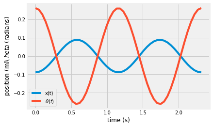
Finally, I find $x(t)$ integrating twice

$x(t) = -\frac{10\theta_0}{\omega^2}\cos\omega t +x_0 +\dot{x}_0 t$

w = np.sqrt(60*m2*9.81*L)
t = np.linspace(0,4*np.pi/w)
theta = np.pi/12*np.cos(w*t)
x = -10*np.pi/12/w**2*np.cos(w*t)

plt.plot(t,x, label = 'x(t)')
plt.plot(t,theta, label = r'$\theta(t)$')

plt.ylabel('position (m)\\ $\theta$ (radians)')
plt.xlabel('time (s)')
plt.legend();

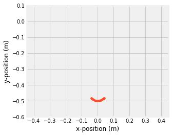
Define the position vectors, $\mathbf{r}_1$ and $\mathbf{r}_2$

r1 = np.block([x[:,np.newaxis],np.zeros((len(x),1))])
r2 = r1 + np.block([L*np.sin(theta[:,np.newaxis]),-L*np.cos(theta[:,np.newaxis])])

from matplotlib import animation
from IPython.display import HTML

fig, ax = plt.subplots()

ax.set_xlim(( x.min()*5, x.max()*5))
ax.set_ylim((-0.6, 0.1))
ax.set_aspect('equal','box')
ax.set_xlabel('x-position (m)')
ax.set_ylabel('y-position (m)')

line, = ax.plot([], [], 's-', markersize =15)
#marker, = ax.plot([], [], 'o', markersize=10)
ax.plot(r2[:,0],r2[:,1],'.')

[<matplotlib.lines.Line2D at 0x7e2379866a30>]

Create an initializing (init) function that clears the previous line and marker

def init():
    line.set_data([], [])
    return (line,)

Create an animating (animate) function that updates the line

def animate(i):
    '''function that updates the line and marker data
    arguments:
    ----------
    i: index of timestep
    outputs:
    --------
    line: the line object plotted in the above ax.plot(...)
    marker: the marker for the end of the 2-bar linkage plotted above with ax.plot('...','o')'''
    line.set_data([r1[i,0], r2[i,0]], [r1[i,1], r2[i,1]])
    return (line, )

Create an animation (anim) variable using the animation.FuncAnimation

anim = animation.FuncAnimation(fig, animate, init_func=init,
                               frames=range(0,len(t)), interval=100, 
                               blit=True)

HTML(anim.to_html5_video())

Advanced Dynamics

Example: Sliding pendulum

Example: Sliding pendulum¶