Embedding technique: solution of link pinned to ground at origin¶

Overview: embedding technique¶

The embedding technique is a generalized method to solve for the dynamic response in a system of moving parts. The generalized coordinates are separated into dependent and independent coordinates as such

\(\mathbf{q} = [\mathbf{q}_d,~\mathbf{q}_i]\).

This distinction creates \(n-n_c\) second order differential equations, where \(n=3\times(\#~bodies)\) and \(n_c=number~of~constraints\). The equations of motion are as such

\(\mathbf{B^TMB +B^TM\gamma-B^TQ_e = 0}\)

where,

\(\mathbf{B}=\left[\begin{array}-\mathbf{C_{q_d}^{-1}C_{q_i}} \\\bar{I}\end{array}\right]\)
\(\gamma = \left[\begin{array} ~\mathbf{-C_{q_d}^{-1}[(C_q\dot{q})_q\dot{q}+2C_{qt}\dot{q}+C_{tt}}] \\ \mathbf{0}\end{array}\right] = \left[\begin{array} ~\mathbf{C_{q_d}^{-1}[Q_d]} \\ \mathbf{0}\end{array}\right]\)
\(\mathbf{C_{q_d}}~and~\mathbf{C_{q_i}}\) are the Jacobian of constraints for dependent and independent coordinates, respectively

System: link pinned to ground¶

link pinned to ground

In the diagram above, a link is pinned to the point \(r_{pin} = x\hat{i}\). In this notebook, you will

build the a single, second order differential equation using the embedded technique
solve the second order differential equation
plot and animate the result

You will define the following functions:

rotA a 2D rotation matrix
A_theta the derivative of rotA
C_link the 2 constraint equations for the link system
Cq_pin the Jacobian of a general pin constraint between 2 rigid bodies
Cq_link the Jacobian of the link system d C_link/dq
Bi_link the array \(\mathbf{B}\) that transforms \(\delta \mathbf{q_i}\) to \(\delta \mathbf{q}\)
eom_bar the final equation of motion using the embedding technique

Define System constants¶

You will use a 1-meter link with mass, m=0.1 kg.

xA = 0 # pin to the origin
m1 = 0.1 # kg
l1 = 1 # m

Define \(\mathbf{A}\) and \(\mathbf{A}_\theta\)¶

Here, you create two functions to rotate from the body coordinate system at angle \(\theta\) to the global coordinate system. The derivate, \(\mathbf{A}_\theta\) will be used in the Jacobian and equations of motion.

def rotA(theta):
    '''This function returns a 2x2 rotation matrix to convert the 
    rotated coordinate to the global coordinate system
    input is angle in radians
        
    Parameters
    ----------
    theta : angle in radians
    
    Returns
    -------
    A : 2x2 array to rotate a coordinate system at angle theta to global x-y
    '''
    A=np.zeros((2,2))
    A=np.array([[np.cos(theta), -np.sin(theta)],
               [np.sin(theta), np.cos(theta)]])
    
    return A

def A_theta(theta):
    '''This function returns a 2x2 rotation matrix derivative 
    input is angle in radians
        
    Parameters
    ----------
    theta : angle in radians
    
    Returns
    -------
    dAda : 2x2 array derivative of `rotA`
    '''
    dAda=np.array([[-np.sin(theta), -np.cos(theta)],
                   [np.cos(theta), -np.sin(theta)]])
    return dAda

Define the constraints \(\mathbf{C}(\mathbf{q},~t)\)¶

There are 2 constraints on the motion and 3 generalized coordinates. The constraint keeps the base of the link at point \(\mathbf{r}_A=x\hat{i}\).

def C_link(q,t):
    '''2 constraint equations for 3 generalized coords
       q=[R1x,R1y,a1]
       q=[R1,     a1]
         [0,1     2 ]
         
              1/
              /     pinned link
             O    
       -----^^^-------------
            
    Parameters
    ----------
    q : numpy array for 9 generalized coordinates for bodies 1-3 in the slider crank
        q = [q1]
    t : current time
    
    Returns
    -------
    C : 2 constraint equation evaluations
    '''
    q1 = q[0:3]
    C=np.zeros(2)
    C[0:2] = q1[0:2]+rotA(q1[2])@np.array([-l1/2, 0]) - np.array([xA, 0])
    return C

Define the Jacobian of constraints \(\mathbf{C}_\mathbf{q}\)¶

There are 2 constraints on the motion and 3 generalized coordinates. The resulting Jacobian is \(2~rows\times 3~columns\). You create a reuseable pin Jacobian (\(2\times 6\)) and use the first three columns in Cq_link.

Define Jacobian of pin constraint as Cq_pin.

def Cq_pin(qi, qj, ui, uj):
    '''Jacobian of a pinned constraint for planar motion

    Parameters
    ----------
    qi : generalized coordinates of the first body, i [Rxi, Ryi, thetai]
    qj : generalized coordinates of the 2nd body, i [Rxj, Ryj, thetaj]
    ui : position of the pin the body-i coordinate system
    uj : position of the pin the body-j coordinate system
        
    Returns
    -------
    Cq_pin : 2 rows x 6 columns Jacobian of pin constraint Cpin
    '''
    
    Cq_1=np.block([np.eye(2), A_theta(qi[2])@ui[:,np.newaxis] ])
    Cq_2=np.block([-np.eye(2), -A_theta(qj[2])@uj[:,np.newaxis] ])
    Cq_pin=np.block([Cq_1, Cq_2])
    return Cq_pin

The bar uses the first three columns of the pin-constraint Jacobian in Cq_link.

def Cq_link(q,t):
    '''return Jacobian of C_slidercrank(q,t) = dC/dq_i
       |dC1/dR1x dC1/dR1y dC1/da3 |
       |dC2/dR1x dC2/dR1y dC2/da3 |
    
    Parameters
    ----------
    q : numpy array for 3 generalized coordinates for body 1 in the rotating link
        q = [q1]
    t : current time
    Returns
    -------
    Cq : 2 rows x 3 columns Jacobian of constraints `C_link`   
    '''
    q1 = q[0:3]
    
    Cq=np.zeros((2,3))
    Cq[0:2, 0:3] = Cq_pin(q1, np.array([0, 0, 0]),np.array([-l1/2, 0]),np.array([0, 0]))[0:2, 0:3]
    return Cq

The g()-function is added to make changing measurement systems easier. You can change to millimeters and seconds or feet and seconds by calling g('mms') or g('fts'), respectively.

def g(system='ms'):
    '''define gravity for m-s, ft-s,mm-s'''
    if system=='ms':
        return 9.81
    elif system=='fts':
        return 32.2
    elif system=='mms':
        return 9.81e3
    else:
        print('warning: system not defined yet, giving you 9.81 m/s/s')
        return 9.81
  

Here, you create the first function for the embedding techique equations of motion

\(\mathbf{B}=[-\mathbf{C_{q_d}^{-1}C_{q_i}},~\bar{I}]^T\)

is defined as function Bi_link(q, t).

Note: In general, you should never invert an array. This is a very rare case when the inverse is strictly necessary. Ideally, you would solve the equation as x = solve(A, b), rather than x = inv(A)@b. In this particular case, \(\mathbf{C_{q_d}}=\mathbf{I}\), so the inverse is \(\mathbf{I}^{-1} = \mathbf{I}\).

def Bi_link(q, t):
    '''B.T*M*B-B.T*Qe = 0 '''
    Cq = Cq_link(q, t)
    Cqd=Cq[0:2,0:2]
    Cqi=Cq[0:2,2].reshape(2,1)
    #print(-np.linalg.inv(Cqd)@Cqi)
    Bi=np.vstack((-np.linalg.inv(Cqd)@Cqi,np.eye(1)))
    return Bi

Solution¶

Solution process:

define a global variable q0 that updates the initial guess for \(\mathbf{C}(\mathbf{q},~t)=\mathbf{0}\)
Use state \(y=[\theta^1,~\dot{\theta}^1]\) to add constraints to \(\mathbf{C}(\mathbf{q},~t)\)
solve for \(y(t)\) using solve_ivp
plug into \(y(t)\) into eom_bar to get generalized coordinates \(\mathbf{q}(t)\)

Define equation of motion¶

The equation of motion for the general embedding method is as such

\(\mathbf{B^TMB +B^TM\gamma-B^TQ_e = 0}\)

\(\gamma = \left[\begin{array} \mathbf{-C_{qd}^{-1}[(C_q\dot{q})_q\dot{q}+2C_{qt}\dot{q}+C_{tt}}] \\ \mathbf{0}\end{array}\right] = \left[\begin{array} \mathbf{C_{qd}^{-1}[Q_d]} \\ \mathbf{0}\end{array}\right]\)

where \(\mathbf{B}=\mathbf{B(q)}\) and \(\mathbf{\gamma = \gamma}(\mathbf{q,~\dot{q},}~t)\). This presents a system of differential algebraic equations. You need to solve for \(\mathbf{q}\) and \(\dot{\mathbf{q}}\) at each step. The one-bar linkage contraints do not invlove time-dependent terms so \(\mathbf{\gamma}=\mathbf{0}\).

Define equation of motion to return \(\dot{y}=[\dot{\theta}^1,~\ddot{\theta}^1]^T\) and \(\mathbf{q}= [R_x^1,~R_y^1,~\theta^1]^T\), where \(y=[\theta^1,~\dot{\theta}^1]^T\).

The equation of motion has a number of steps to get to the final result. Notice the solution for q. The values of \(q_1=R_x^1\) and \(q_2=R_y^1\) depend upon \(q_3=\theta^1\), but \(\theta^1\) is the unknown independent generalized coordinate.

q = fsolve(lambda q: np.block([C_link(q, t), q[2] - y[0]]), q0, \
                  fprime= lambda q: np.vstack((Cq_link(q,t), np.array([0,0,1]))))

This fsolve solution creates a third constraint that \(\theta^1 =\) y[0] the first state variable. The added constraint changes the dimensions of the Jacobian

\(\mathbf{C}(\mathbf{q},~t) = \left[\mathbf{R}^1+\mathbf{Au}_A-\mathbf{r}_A \right] \rightarrow \left[\begin{array}{c}~\mathbf{R}^1+\mathbf{Au}_A-\mathbf{r}_A \\ \theta^1 - y[0] \end{array} \right]\)
\(\mathbf{C}_\mathbf{q} = \left[\begin{array}{c}~1 & 0 & \frac{l^1}{2}\sin\theta^1 \\ 0 & 1 & -\frac{l^1}{2}\cos\theta^1 \end{array} \right] \rightarrow \left[\begin{array}{c}~1 & 0 & \frac{l^1}{2}\sin\theta^1 \\ 0 & 1 & -\frac{l^1}{2}\cos\theta^1 \\ 0 & 0 & 1 \end{array}\right]\)

The function eom_bar calculates -dy: \(\frac{dy}{dt}\) -q: \(\mathbf{q}\).

q0=np.array([l1/2, 0, 0])

def eom_bar(t, y, li = l1, mi = m1):
    '''    
    Parameters
    ----------
    ti : current time
    y : numpy array for independent generalized coordinates for body 1 in the rotating link
        y = [theta, dtheta/dt]
    
    global parameter:
    -----------------
    q0 : initial guess to solve C(q, t) equations
    
    Returns
    -------
    dy : derivative for the independent generalized coordinate for body 1
         dy = [dtheta/dt, ddtheta/ddt]
    '''
    global q0
    
    q0[2]=y[0]
    
    q = fsolve(lambda q: np.block([C_link(q, t),q[2]-y[0]]),q0, \
                  fprime= lambda q: np.vstack((Cq_link(q,t),np.array([0,0,1]))))
    
    Bi = Bi_link(q, t)
    M = np.diag([mi,mi,mi*li**2/12])
    Qe = np.array([0, -mi*g(), 0])
    dy = np.zeros(y.shape)
    dy[0] = y[1]
    dy[1] = solve(Bi.T@M@Bi,Bi.T@Qe)
    return dy, q

Solve for \(\theta^1(t)\)¶

The value of \(\mathbf{q}\) is needed to calculate \(\mathbf{C_q}\) and \(\mathbf{B}\), but in the first pass to get a solution for the \(\theta^1(t)\), you ignore the values of q by indexing the eom_bar function as such

lambda t, y: eom_bar(t, y)[0] # <-- only grab the first output from eom_bar

You will solve for the motion of the link starting from rest with initial conditions, \([\theta,~\dot{\theta}] = [0~rad,~0~rad/s]\).

t = np.linspace(0,4)
sol=solve_ivp(lambda t, y: eom_bar(t, y)[0], 
              t_span = [0,t.max()], 
              y0 = [0, 0], 
              t_eval = t)

Verify work¶

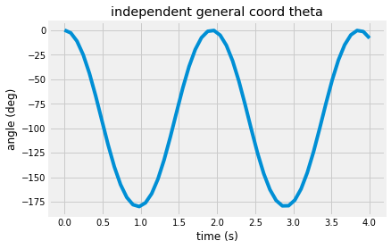
You should expect oscillations with magnitude \(180^o\) around the equilibrium position at \(-90^o\).

plt.plot(sol.t,sol.y[0]*180/np.pi)

plt.xlabel('time (s)')
plt.ylabel('angle (deg)')
plt.title('independent general coord theta')

Text(0.5, 1.0, 'independent general coord theta')

Solve for \(\mathbf{q}(t)\)¶

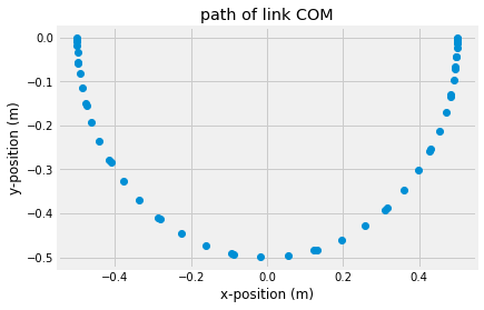
Plug in the solution sol.y for \(\mathbf{q}\) as a function of time to get the other generalized coordinates.

q=np.zeros((3,len(t)))
for i,ti in enumerate(t):
    dy, qi = eom_bar(ti,sol.y[:,i])
    q[:,i] = qi

plt.plot(q[0,:],q[1,:], 'o')
plt.xlabel('x-position (m)')
plt.ylabel('y-position (m)')
plt.title('path of link COM')

Text(0.5, 1.0, 'path of link COM')

Animate the motion¶

Next, you animate the motion of the system. Below, you create

plot_shape to create lines and markers to represent links and the sliding base
a figure that shows the path of the two link centers of mass 3.init to initialize the animation
animate to update the two links and sliding base
FuncAnimation to display the motion of the slidercrank system

def plot_shape(shape,dims,q):
    '''
    function to plot a shape based upon the shape dimensions and coordinates
    arguments:
    ----------
    shape: either 'link' or 'base',
            - the link returns two points to plot as a line
            - the base returns one point to plot as a marker
            - if neither 'link' or 'base' are chosen, then 0 is returned and warning printed 
            `choose a \'link\' or \'base\' please`
    dims: the dimensions of the shape
            - the link uses the first value as the length
            - the base ignores the `dims`
    q: generalized coordinates in the form [Rx, Ry, theta]
            - the link returns the center of the link at (Rx, Ry) and oriented at theta
            - the base returns the center at (Rx, Ry) and ignores theta
    returns:
    --------
    datax: coordinates to plot the x-positions
    datay: coordinates to plot the y-positions
            - the link returns array of length 2
            - the base returns array of length 1
    
    '''

    if shape=='link':
        left = rotA(q[2])@np.array([-dims[0]/2, 0])
        right = rotA(q[2])@np.array([dims[0]/2, 0])
        Px=q[0]+np.array([left[0], right[0]])
        Py=q[1]+np.array([left[1], right[1]])
        datax = Px
        datay = Py
        #l,= plt.plot(Px,Py,'o-')
        return datax, datay
    elif shape=='base':
        Px=q[0]
        Py=q[1]
        data = [Px, Py]
        #l,=plt.plot(Px,Py,'s',markersize=20)
        return data
    else:
        print('choose a \'link\' or \'base\' please')
        return 0

2. initialize the lines and coordinate system¶

q1 = q[0:3, :]

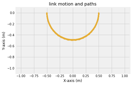
fig, ax = plt.subplots()
link1, = ax.plot([], [], linewidth = 10)
body3, = ax.plot([], [], 's', markersize = 20)
path1, = ax.plot(q1[0, :], q1[1, :])
ax.set_xlim((-1.1,1.1))
ax.set_ylim((-1.1, 0.1))
ax.set_xlabel('X-axis (m)')
ax.set_ylabel('Y-axis (m)')
ax.set_title('link motion and paths')

Text(0.5, 1.0, 'link motion and paths')

3. and 4. create your `init` and `animation` functions to update the lines on the plot¶

Create an initializing (init) function that clears the previous lines and markers

Create an animating (animate) function that updates the link, base, and path

def init():
    link1.set_data([], [])
    return (link1, )

def animate(i):
    '''function that updates the line and marker data
    arguments:
    ----------
    i: index of timestep
    outputs:
    --------
    link1: the line object plotted in the above ax.plot(...)
    '''

    datax, datay = plot_shape('link', np.array([l1]), q1[:, i])
    link1.set_data(datax, datay)
    
    return (link1, )

4. display the result in an HTML video¶

Import the animation and HTML functions. Then, create an animation (anim) variable using the animation.FuncAnimation

from matplotlib import animation
from IPython.display import HTML

anim = animation.FuncAnimation(fig, animate, init_func=init,
                               frames=range(0,len(t)), interval=50, 
                               blit=True)

HTML(anim.to_html5_video())

Advanced Dynamics

Embedding technique: solution of link pinned to ground at origin

Contents

Embedding technique: solution of link pinned to ground at origin¶

Overview: embedding technique¶

System: link pinned to ground¶

Define System constants¶

Define \(\mathbf{A}\) and \(\mathbf{A}_\theta\)¶

Define the constraints \(\mathbf{C}(\mathbf{q},~t)\)¶

Define the Jacobian of constraints \(\mathbf{C}_\mathbf{q}\)¶

Solution¶

Define equation of motion¶

Solve for \(\theta^1(t)\)¶

Verify work¶

Solve for \(\mathbf{q}(t)\)¶

Animate the motion¶

2. initialize the lines and coordinate system¶

3. and 4. create your `init` and `animation` functions to update the lines on the plot¶

4. display the result in an HTML video¶

Advanced Dynamics

Embedding technique: solution of link pinned to ground at origin

Contents

Embedding technique: solution of link pinned to ground at origin¶

Overview: embedding technique¶

System: link pinned to ground¶

Define System constants¶

Define \(\mathbf{A}\) and \(\mathbf{A}_\theta\)¶

Define the constraints \(\mathbf{C}(\mathbf{q},~t)\)¶

Define the Jacobian of constraints \(\mathbf{C}_\mathbf{q}\)¶

Solution¶

Define equation of motion¶

Solve for \(\theta^1(t)\)¶

Verify work¶

Solve for \(\mathbf{q}(t)\)¶

Animate the motion¶

2. initialize the lines and coordinate system¶

3. and 4. create your init and animation functions to update the lines on the plot¶

4. display the result in an HTML video¶

3. and 4. create your `init` and `animation` functions to update the lines on the plot¶