Example: Describing 3D circular motion¶

In this example, a particle is traveling in a circle around an axis set to \(\hat{e}_{rot} = -\frac{1}{\sqrt{2}}\hat{i}+\frac{1}{\sqrt{2}}\hat{k}\).

I create a rotation: \(R_1\) to rotate the unit vector around the \(\hat{j}\)-axis by \(45^o\).

I want to rotate the starting position of the position by \(60^o\) so the particle didn’t start along one of the axes. This rotation is \(R_2\).

alpha = np.pi/4; R1 = np.array([[np.cos(alpha), 0, -np.sin(alpha)],
                                [0,1,0],
                                [np.sin(alpha), 0, np.cos(alpha)]])
beta = np.pi/3; R2 = np.array([[np.cos(beta), -np.sin(beta), 0],
                               [np.sin(beta), np.cos(beta), 0],
                               [0,0,1]])

Next, I define the angle to go through one cycle,a= \(\theta=0-2\pi\) and defined the \(r'\) and \(v'\) vectors.

a = np.linspace(0,2*np.pi)
rp = np.array([np.sin(a), np.cos(a), np.zeros(a.shape)])
vp = np.array([np.cos(a), -np.sin(a), np.zeros(a.shape)])

Rotating \(\mathbf{r}'\) and \(\mathbf{v}'\) to the desired coordinates required multiplying the rotation matrices as such

\(\mathbf{r} = \mathbf{R_1R_2r}'\)
\(\mathbf{v} = \mathbf{R_1R_2v}'\)

r = rp.copy()
v = vp.copy()
for i in range(0,len(a)):
    r[:,i] = R1@R2@rp[:,i]
    v[:,i] = R1@R2@vp[:,i]

Then, I print out the values for \(\mathbf{r}(0)\), \(\mathbf{v}(0)\), and \(\mathbf{h}(0)\)

print(1*r[:,0])
print(1*v[:,0])
h = np.cross(r[:,0],v[:,0])
print(h)

[-0.61237244  0.5        -0.61237244]
[0.35355339 0.8660254  0.35355339]
[ 0.70710678  0.         -0.70710678]

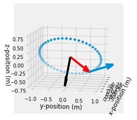
Finally, to give context I plot the motion of the object with the three vectors plotted

\(\mathbf{r}(0)\): red
\(\mathbf{v}(0)\): blue
\(\mathbf{h}(0)\): black

fig = plt.figure()
ax = fig.add_subplot(111, projection='3d')
ax.scatter(r[0,:],r[1,:],r[2,:])
Q1 = ax.quiver(r[0,0],r[1,0],r[2,0], v[0,0],v[1,0],v[2,0])
Q2 = ax.quiver(0,0,0, r[0,0],r[1,0],r[2,0],color='red')
Q3 = ax.quiver(0,0,0,h[0],h[1],h[2],color='black')
ax.view_init(elev=10., azim=10)
ax.set_xlabel('x-position (m)')
ax.set_ylabel('y-position (m)')
ax.set_zlabel('z-position (m)')

Text(0.5, 0, 'z-position (m)')

from matplotlib import animation
from IPython.display import HTML

Create a figure to display the animation and add fixed background the dashed line is added to show the path the end point takes

Create an initializing (init) function that clears the previous line and marker

def init():
    Q1.set_UVC([], [], [])
    Q2.set_UVC([], [], [])
    Q3.set_UVC([], [], [])
    return (Q1, Q2, Q3,)

Create an animating (animate) function that updates the line

def animate(i):
    '''function that updates the line and marker data
    arguments:
    ----------
    i: index of timestep
    outputs:
    --------
    line: the line object plotted in the above ax.plot(...)
    marker: the marker for the end of the 2-bar linkage plotted above with ax.plot('...','o')'''
    Q1.set_UVC = ax.quiver(r[0,i],r[1,i],r[2,i], v[0,i],v[1,i],v[2,i])
    Q2.set_UVC = ax.quiver(0,0,0, r[0,i],r[1,i],r[2,i],color='red')
    h = np.cross(r[:,i],v[:,i])
    Q3.set_UVC = ax.quiver(0,0,0,h[0],h[1],h[2],color='black')
    return (Q1, Q2, Q3, )

Create an animation (anim) variable using the animation.FuncAnimation

anim = animation.FuncAnimation(fig, animate, #init_func=init,
                               frames=range(0,len(a)), interval=100, 
                               blit=False)

HTML(anim.to_html5_video())

Advanced Dynamics

Example: Describing 3D circular motion

Example: Describing 3D circular motion¶