Homework #1
Contents
import numpy as np
from numpy import sin,cos,pi
import matplotlib.pyplot as plt
plt.style.use('fivethirtyeight')
Homework #1
Example: plotting kinematic solutions
define kinematic known values
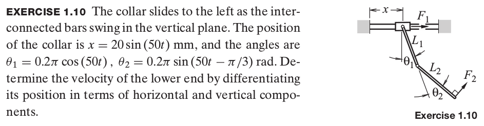
First, we can define the independent variable, t, to complete one full cycle. Then, we can use the inputs for \(x,~\theta_1,~and~\theta_2\).
t=np.linspace(0,2*pi/50,100); # create time varying from 0-0.126 s (or one period)
x=20*sin(50*t);     # define x in terms of time
dx=20*50*cos(50*t); # define dx/dt in terms of time (note dx=dx/dt)
t1=0.2*pi*cos(50*t); # define theta1 (t1)
dt1=-10*pi*sin(50*t); # define dtheta1/dt (dt1)
t2=0.2*pi*sin(50*t-pi/3); # define theta2 (t2) ;
dt2=10*pi*sin(50*t-pi/3); # define dtheta2/dt (dt2);
L1=1;L2=1.5; # set lengths for L1 and L2 (none were given in problem so 1 and 1.5 mm were
             # chosen arbitrarily
define the other dependent kinematic values
In the lecture, you derived the positions of the link connections using the given values. Here, we apply those definitions to get the global positions of each link endpoint.
rcc=np.array([x+L1*sin(t1),-L1*cos(t1)]) # position of connection between links
rco=np.array([x+L1*sin(t1)+L2*sin(t2),-(L1*cos(t1)+L2*cos(t2))])    # create a row vectors of
                                                                    # x-component and y-component of
                                                                    # pendulum position C (r_C/O)
vco=np.array([dx+L1*cos(t1)*dt1+L2*cos(t2)*dt2,
     (L1*sin(t1)*dt1+L2*sin(t2)*dt2)]) # create row
                                       # vectors of
                                       # the x- and
                                       # y-component
                                       # velocity of
                                       # point C
Plot results
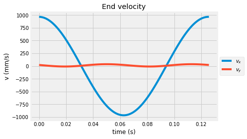
Here, you plot the velocity components of the end of the lower link.
plt.plot(t,vco[0,:],label=r'$v_x$')
plt.plot(t,vco[1,:],label=r'$v_y$')
plt.xlabel('time (s)')
plt.ylabel('v (mm/s)')
plt.legend(loc='center left', bbox_to_anchor=(1, 0.5))
plt.title('End velocity')
Text(0.5, 1.0, 'End velocity')
Animate the motion
Here, you create an HTML animation for the 2-bar linkage
Create function that plots the links at timesteps
from matplotlib import animation
from IPython.display import HTML
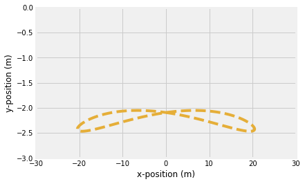
Create a figure to display the animation and add fixed background the dashed line is added to show the path the end point takes
fig, ax = plt.subplots()

ax.set_xlim(( -30, 30))
ax.set_ylim((-3, 0))
ax.set_xlabel('x-position (m)')
ax.set_ylabel('y-position (m)')

line, = ax.plot([], [])
marker, = ax.plot([], [], 'o', markersize=10)
ax.plot(rco[0,:],rco[1,:],'--')
[<matplotlib.lines.Line2D at 0x74b421c5cb80>]
Create an initializing (
init) function that clears the previous line and marker
def init():
    line.set_data([], [])
    marker.set_data([], [])
    return (line,marker,)
Create an animating (
animate) function that updates the line
def animate(i):
    '''function that updates the line and marker data
    arguments:
    ----------
    i: index of timestep
    outputs:
    --------
    line: the line object plotted in the above ax.plot(...)
    marker: the marker for the end of the 2-bar linkage plotted above with ax.plot('...','o')'''
    line.set_data([x[i],rcc[0,i],rco[0,i]],[0,rcc[1,i],rco[1,i]])
    marker.set_data([rco[0, i], rco[1,i]])
    return (line, marker, )
Create an animation (
anim) variable using theanimation.FuncAnimation
anim = animation.FuncAnimation(fig, animate, init_func=init,
                               frames=range(0,len(t)), interval=100,
                               blit=True)
HTML(anim.to_html5_video())
Problem 1
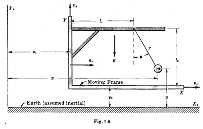
The axis shown in Fig 1-5 has the following constants
\(v_x=5\) m/s.
\(m= 0.5\) kg
\(r= 0.75\) m
\(l_2 = 1\) m
\(l_1 = 1.5\) m
\(s_2 = 0.1\) m
\(v_y = 0\) m/s
\(a_x = 0~m/s^2~or~5~m/s^2\)
(a) Plot the angle of the pendulum for one full period of oscillation given \(\theta(0)=\pi/18\) and \(\dot{\theta}(0)=0\)
(b) Plot the global path of the object in terms of \(X_1\) and \(X_2\) for \(t=0-2\)s for both
\(a_x=\) 0 m/s\(^2\)
\(a_x=\) 5 m/s\(^2\)
(c) Plot the angle \(\theta\) for one period of oscillation for 2 conditions, label your two lines on one graph:
\(a_x=\) 0 m/s\(^2\)
\(a_x=\) 5 m/s\(^2\)