Numerical Error
Contents
Numerical Error
Content modified under Creative Commons Attribution license CC-BY 4.0, code under BSD 3-Clause License © 2020 R.C. Cooper
Freefall Model Computational solution
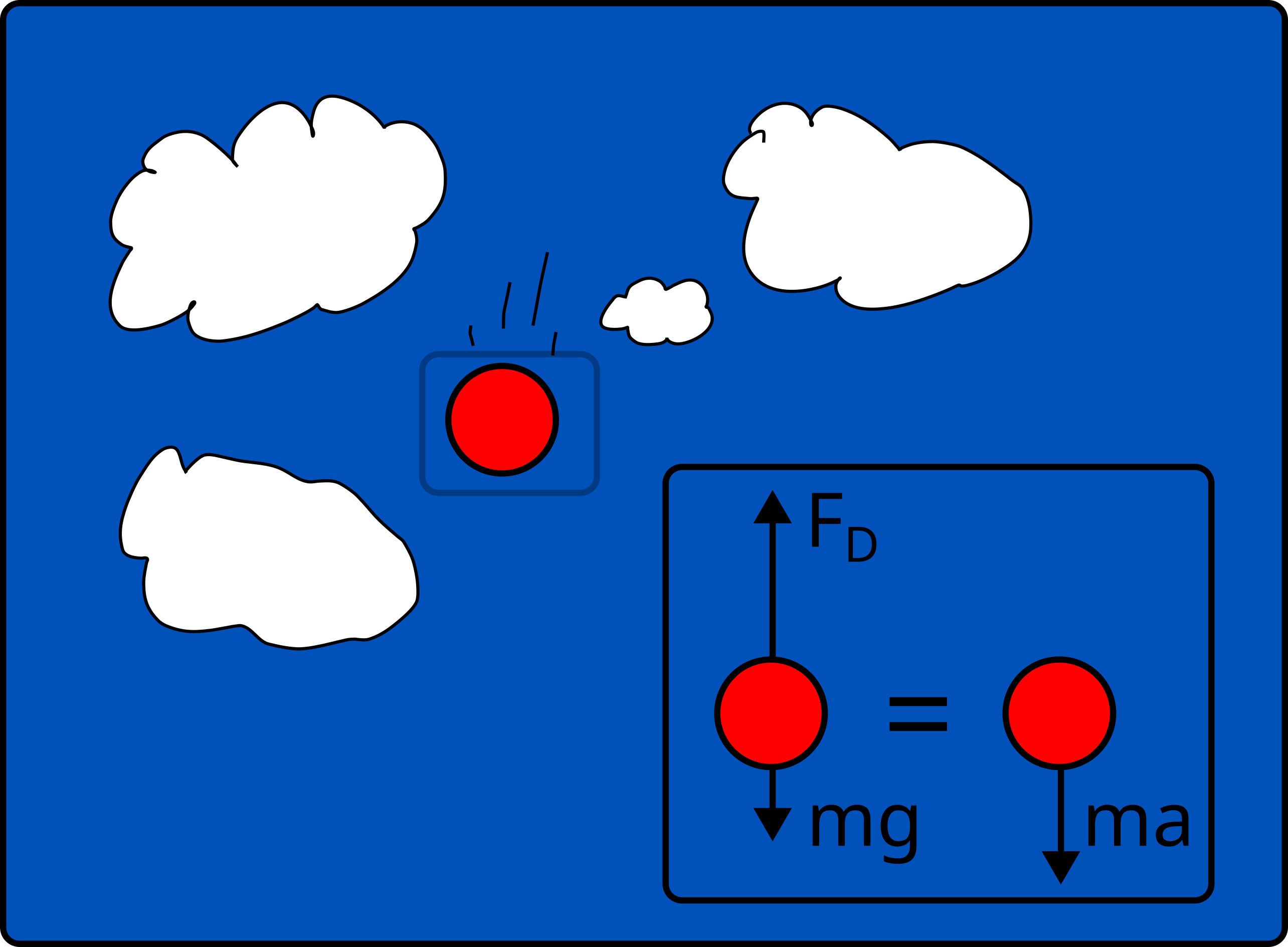
Here is our first computational mechanics model.
An object falling is subject to the force of
gravity (\(F_g\)=mg) and
drag (\(F_d=cv^2\))
Acceleration of the object:
\(\sum F=ma=F_g-F_d=mg - cv^2 = m\frac{dv}{dt}\)
Define constants and analytical solution (meters-kilogram-sec)
We define parameters for our problem as the acceleration due to gravity, g, drag coefficient, c, and mass of the object, m. Once we have defined these parameters, we have a single variable whose derivative \(\frac{dv}{dt}\) is equal to a function of itself \(v\) i.e. \(\frac{dv}{dt} = f(v,~parameters)\).
parameters:
g=9.81 m/s\(^2\), c=0.25 kg/m, m=60 kg
function:
\(\frac{dv}{dt} = g-\frac{c}{m}v^2\)
We can solve for the analytical solution in this case. First, consider the speed of the falling object when acceleration is \(\frac{dv}{dt}=0\), this is called the terminal velocity, \(v_{terminal}\).
\(v_{terminal}=\sqrt{\frac{mg}{c}}\)
Now, substitute this terminal velocity into the equation and integrate to get the analytical solution v(t):
\(v(t)=v_{terminal}\tanh{\left(\frac{gt}{v_{terminal}}\right)}\).
import numpy as np
import matplotlib.pyplot as plt
Exercise:
Calculate the terminal velocity for the given parameters, g=9.81 m/s\(^2\), c=0.25 kg/m, m=60 kg.
c=0.25
m=60
g=9.81


def v_analytical(t,m,g,c):
    '''Analytical solution for the velocity of an object released from rest subject to
    the force of gravity and the force of drag with drag coefficient, c

        Arguments
    ---------
    t: time, the independent variable
    m: mass of the object
    g: acceleration due to gravity
    c: drag coefficient

    Returns
    -------
    v: the speed of the object at time t'''

    v_terminal=np.sqrt(m*g/c)
    v= v_terminal*np.tanh(g*t/v_terminal)
    return v
Inside the curly brackets¿the placeholders for the values we want to print¿the f is for float and the .4 is for four digits after the decimal dot. The colon here marks the beginning of the format specification (as there are options that can be passed before). There are so many tricks to Python’s string formatter that you’ll usually look up just what you need.
Another useful resource for string formatting is the Python String Format Cookbook. Check it out!
If we print these values using the string formatter, with a total length of 5 and only printing 2 decimal digits, we can display our solution in a human-readable way.
{:5.2f}
where
:5prints something with whitespace that is 5 spaces total.2prints 2 significant figures after the decimalftellsformatthat the input is a floating point number to print
for t in range(0,14,2):
    print('at time {:5.2f} s, speed is {:5.2f} m/s'.format(t,v_analytical(t,m,g,c)))
at time  0.00 s, speed is  0.00 m/s
at time  2.00 s, speed is 18.62 m/s
at time  4.00 s, speed is 32.46 m/s
at time  6.00 s, speed is 40.64 m/s
at time  8.00 s, speed is 44.85 m/s
at time 10.00 s, speed is 46.85 m/s
at time 12.00 s, speed is 47.77 m/s
Analytical vs Computational Solution
The analytical solution above gives us an exact function for \(v(t)\). We can input any time, t, and calculate the speed, v.
In many engineering problems, we cannot find or may not need an exact mathematical formula for our design process. It is always helpful to compare a computational solution to an analytical solution, because it will tell us if our computational solution is correct. Next, we will develop the Euler approximation to solve the same problem.
Define numerical method
Finite difference approximation
Computational models do not solve for functions e.g. v(t), but rather functions at given points in time (or space). In the given freefall example, we can approximate the derivative of speed, \(\frac{dv}{dt}\), as a finite difference, \(\frac{\Delta v}{\Delta t}\) as such,
\(\frac{v(t_{i+1})-v(t_{i})}{t_{i+1}-t_{i}}=g-\frac{c}{m}v(t_{i})^2\).
Then, we solve for \(v(t_{i+1})\), which is the velocity at the next time step
\(v(t_{i+1})=v(t_{i})+\left(g-\frac{c}{m}v(t_{i})^2\right)(t_{i+1}-t_{i})\)
or
\(v(t_{i+1})=v(t_{i})+\frac{dv_{i}}{dt}(t_{i+1}-t_{i})\)
Now, we have function that describes velocity at the next timestep in terms of a current time step. This finite difference approximation is the basis for a number of computational solutions to ordinary and partial differential equations.
Therefore, when we solve a computational problem we have to choose which points in time we want to know the velocity. To start, we define time from 0 to 12 seconds
t=[0,2,4,6,8,10,12]
import numpy as np
#t=np.array([0,2,4,6,8,10,12])
# or
t=np.linspace(0,12,7)
Now, we create a for-loop to solve for v_numerical at times 2, 4, 6, 8, 10, and 12 sec. We don’t need to solve for v_numerical at time 0 seconds because this is the initial velocity of the object. In this example, the initial velocity is v(0)=0 m/s.
v_numerical=np.zeros(len(t));
for i in range(1,len(t)):
    v_numerical[i]=v_numerical[i-1]+((g-c/m*v_numerical[i-1]**2))*2;

v_numerical
array([ 0.        , 19.62      , 36.03213   , 44.8328434 , 47.702978  ,
       48.35986042, 48.49089292])
Let’s print the time, velocity (analytical) and velocity (numerical) to compare the results in a table. We’ll use the print and format commands to look at the results.
print('time (s)|vel analytical (m/s)|vel numerical (m/s)')
print('-----------------------------------------------')
for i in range(0,len(t)):
    print('{:7.1f} | {:18.2f} | {:15.2f}\n'.format(t[i],v_analytical(t[i],m,g,c),v_numerical[i]));
time (s)|vel analytical (m/s)|vel numerical (m/s)
-----------------------------------------------
    0.0 |               0.00 |            0.00

    2.0 |              18.62 |           19.62

    4.0 |              32.46 |           36.03

    6.0 |              40.64 |           44.83

    8.0 |              44.85 |           47.70

   10.0 |              46.85 |           48.36

   12.0 |              47.77 |           48.49
Compare solutions (plotting)
We can compare solutions in a figure in a number of ways:
plot the values, e.g. \(v_{analytical}\) and \(v_{numerical}\)
plot the difference between the values (the absolute error) e.g. \(v_{numerical}-v_{analytical}\)
plot the ratio of the values e.g. \(\frac{v_{numerical}}{v_{analytical}}\) (useful in finding bugs, unit analysis, etc.)
plot the ratio of the error to the best estimate (the relative error) e.g. \(\frac{v_{numerical}-v_{analytical}}{v_{analytical}}\)
Let’s start with method (1) to compare our analytical and computational solutions.
Import pyplot and update the default plotting parameters.
import matplotlib.pyplot as plt

plt.rcParams.update({'font.size': 22})
plt.rcParams['lines.linewidth'] = 3
plt.plot(t,v_analytical(t,m,g,c),'-',label='analytical')
plt.plot(t,v_numerical,'o-',label='numerical')
plt.legend()
plt.xlabel('time (s)')
plt.ylabel('velocity (m/s)')
Text(0, 0.5, 'velocity (m/s)')
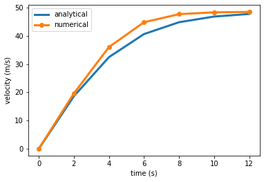
Note: In the above plot, the numerical solution is given at discrete points connected by lines, while the analytical solution is drawn as a line. This is a helpful convention. We plot discrete data such as numerical solutions or measured data as points and lines while analytical solutions are drawn as lines.
Exercise
Play with the values of t (defined above as t=np.linspace(0,12,7)).
If you increase the number of time steps from 0 to 12 seconds what happens to v_analytical? to v_numerical?
What happens when you decrease the number of time steps?
1- Truncation error
Freefall is example of “truncation error”
Truncation error results from approximating exact mathematical procedure
We approximated the derivative as \(\frac{d v}{d t}\approx\frac{\Delta v}{\Delta t}\)
Can reduce error in two ways
Decrease step size -> \(\Delta t\)=
delta_timeIncrease the accuracy of the approximation
Truncation error as a Taylor series
The freefall problem solution used a first-order Taylor series approximation
Taylor series: \(f(x)=f(a)+f'(a)(x-a)+\frac{f''(a)}{2!}(x-a)^{2}+\frac{f'''(a)}{3!}(x-a)^{3}+...\)
First-order approximation: \(f(x_{i+1})=f(x_{i})+f'(x_{i})h\)
We can increase accuracy in a function by adding Taylor series terms:
Approximation |
formula |
|---|---|
\(0^{th}\)-order |
\(f(x_{i+1})=f(x_{i})+R_{1}\) |
\(1^{st}\)-order |
\(f(x_{i+1})=f(x_{i})+f'(x_{i})h+R_{2}\) |
\(2^{nd}\)-order |
\(f(x_{i+1})=f(x_{i})+f'(x_{i})h+\frac{f''(x_{i})}{2!}h^{2}+R_{3}\) |
\(n^{th}\)-order |
\(f(x_{i+1})=f(x_{i})+f'(x_{i})h+\frac{f''(x_{i})}{2!}h^{2}+...\frac{f^{(n)}}{n!}h^{n}+R_{n}\) |
Where \(R_{n}=O(h^{n+1})\) is the error associated with truncating the approximation at order \(n\).
In the .gif below, the error in the function is reduced by including higher-order terms in the Taylor series approximation.
\(n^{th}\)-order approximation equivalent to an \(n^{th}\)-order polynomial.
2- Roundoff
Just storing a number in a computer requires rounding
In our analytical solution, \(v(t) = v_{terminal}\tanh{\left(\frac{gt}{v_{terminal}}\right)}\), we can solve for velocity, \(v\) at any given time, \(t\) by hand to avoid roundoff error, but this is typically more trouble than its worth. Roundoff error comes in two forms:
digital representation of a number is rarely exact
arithmetic (+,-,/,*) causes roundoff error
digital representation of \(\pi\)
Consider the number \(\pi\). How many digits can a floating point number in a computer accurately represent?
pi=np.pi

double=np.array([pi],dtype='float64')
single=np.array([pi],dtype='float32')
print('double precision 64 bit pi = {:1.27f}'.format(double[0])) # 64-bit
print('single precision 32 bit pi = {:1.27f}'.format(single[0])) # 32-bit
print('First 27 digits of pi      = 3.141592653589793238462643383')
double precision 64 bit pi = 3.141592653589793115997963469
single precision 32 bit pi = 3.141592741012573242187500000
First 27 digits of pi      = 3.141592653589793238462643383
In order to store the number in a computer you can only use so many bits, shown below is the 64-bit standard for floating point numbers:

Where the sign is either + or -, the exponent is a power of two as in, \(2^{exponent}\), and the fraction (or base) is the binary representation of the number, \(1+\sum_{i=1}^{52}b_i2^{-i}\). We examine the floating point number representation to highlight that any number you store in a computer is an approximation of the real number you are trying to save. With 64-bit floating point numbers, these approximations are extremely good.
Floating point arithmetic
Each time you use an operation, e.g. + - / * you lose some precision as well.
Consider \(\pi\) again, but this time we will use a for loop to multiply \(\pi\) by a 1e-16 then divide by 1e-16, then multiply by 2e-16 and divide by 2e-16, and so on until we reach 10e-16. If we do these calculations by hand, we see that each step in the for loop returns \(\pi\), but due to floating point arithmetic errors we accumulate some error.
double=np.array([pi],dtype='float64')
double_operated=double
for i in range(0,10):
    double_operated=double_operated*(i+1)*1.0e-16
    double_operated=double_operated*1/(i+1)*1.0e16
print(' 0 operations 64 bit pi = %1.26f\n'%double) # 64-bit
print('20 operations 64 bit pi = %1.26f\n'%double_operated) # 64-bit after 1000 additions and 1 subtraction
print('First 26 digits of pi   = 3.14159265358979323846264338')
 0 operations 64 bit pi = 3.14159265358979311599796347

20 operations 64 bit pi = 3.14159265358979089555191422

First 26 digits of pi   = 3.14159265358979323846264338
In the previous block of code, we see \(\pi\) printed for 3 cases:
the 64-bit representation of \(\pi\)
the value of \(\pi\) after it has gone through 20 math operations (\(\times (0..10)10^{-16}\), then \(\times 1/(0..10)10^{16}\))
the actual value of \(\pi\) for the first 26 digits
All three (1-3) have the same first 14 digits after the decimal, then we see a divergence between the actual value of \(\pi\) (3), and \(\pi\) as represented by floating point numbers.
We can get an idea for computational limits using some built-in functions:
np.info('float64').max: the largest floating point 64-bit number the computer can representnp.info('float64').tiny: the smallest non-negative 64-bit number the computer can representnp.info('float64').eps: the smallest number that can be added to 1
print('realmax = %1.20e\n'%np.finfo('float64').max)
print('realmin = %1.20e\n'%np.finfo('float64').tiny)
print('maximum relative error = %1.20e\n'%np.finfo('float64').eps)
realmax = 1.79769313486231570815e+308

realmin = 2.22507385850720138309e-308

maximum relative error = 2.22044604925031308085e-16
Machine epsilon
The smallest number that can be added to 1 and change the value in a computer is called “machine epsilon”, \(eps\). If your numerical results are supposed to return 0, but instead return \(2eps\), have a drink and move on. You won’t get any closer to your result.
In the following example, we will add \(eps/2\) 1,000\(\times\) to the variable s, set to 1. The result should be \(s=1+500\cdot eps\), but because \(eps/2\) is smaller than floating point operations can track, we will get a different result depending upon how we do the addition.
a. We make a for-loop and add \(eps/2\) 1000 times in the loop
b. We multiply \(1000*eps/2\) and add it to the result
s1=1;
N=1000
eps=np.finfo('float64').eps
for i in range(1,N):
    s1+=eps/2;

s2=1+500*eps
print('summation 1+eps/2 over ',N,' minus 1 =',(s-1))
print(N/2,'*eps=',(s2-1))
---------------------------------------------------------------------------
NameError                                 Traceback (most recent call last)
Input In [12], in <cell line: 8>()
      5     s1+=eps/2;
      7 s2=1+500*eps
----> 8 print('summation 1+eps/2 over ',N,' minus 1 =',(s-1))
      9 print(N/2,'*eps=',(s2-1))

NameError: name 's' is not defined
Exercise
Try adding \(2eps\) to 1 and determine the result of the previous exercise.
What is machine epsilon for a 32-bit floating point number?
Freefall Model (revisited)
In the following example, we judge the convergence of our solution with the new knowledge of truncation error and roundoff error.
The definition for convergence in mathematics is the limit of a sequence exists.
In the case of the Euler approximation, the sequence is smaller timesteps, \(\Delta t\), should converge to the analytical solution.
Define time from 0 to 12 seconds with N timesteps
function defined as freefall
m=60 kg, c=0.25 kg/m
Freefall example
Estimated the function with a \(1^{st}\)-order approximation, so
\(v(t_{i+1})=v(t_{i})+v'(t_{i})(t_{i+1}-t_{i})+R_{1}\)
\(v'(t_{i})=\frac{v(t_{i+1})-v(t_{i})}{t_{i+1}-t_{i}}-\frac{R_{1}}{t_{i+1}-t_{i}}\)
\(\frac{R_{1}}{t_{i+1}-t_{i}}=\frac{v''(\xi)}{2!}(t_{i+1}-t_{i})\)
or the truncation error for a first-order Taylor series approximation is
\(R_{1}=O(\Delta t^{2})\)
Computer model error = truncation + roundoff
In the function freefall(N), the speed of a 60-kg object is predicted in two ways:
The analytical 64-bit representation, \(v(t)=v_{terminal}\tanh{\left(\frac{gt}{v_{terminal}}\right)}\)
The numerical 32-bit\(^{+}\) Euler approximation for
N-steps from 0 to 2 seconds
\(^{+}\)Here, we use a 32-bit representation to observe the transition from truncation error to floating point error in a reasonable number of steps.
We can reduce truncation error by decreasing the timestep, \(\Delta t\). Here, we consider the speed from 0 to 2 seconds, so N=3 means \(\Delta t\)= 1 s and N=21 means \(\Delta t\)=0.1 s
N= |
\(\Delta t\)= |
|---|---|
3 |
1 s |
21 |
0.1 s |
201 |
0.01 s |
?? |
0.05 s |
?? |
0.001 s |
What is N for 0.05 s and 0.001 s in the table above?
Answer (0.05 s): 41
Answer (0.001 s): 2001
Highlight lines above for answer.
def freefall(N):
    '''  help file for freefall(N)
         computes the velocity as a function of time, t, for a
         60-kg object with zero initial velocity and drag
         coefficient of 0.25 kg/s
         N is number of timesteps between 0 and 2 sec
         v_analytical is the 64-bit floating point "true" solution
         v_numerical is the 32-bit approximation of the velocity
         t is the timesteps between 0 and 2 sec, divided into N steps'''
    t=np.linspace(0,2,N)
    c=0.25
    m=60
    g=9.81
    v_terminal=np.sqrt(m*g/c)

    v_analytical = v_terminal*np.tanh(g*t/v_terminal);
    v_numerical=np.empty(len(t),dtype=np.float32)
    delta_time =np.diff(t)
    for i in range(0,len(t)-1):
        v_numerical[i+1]=v_numerical[i]+(g-c/m*v_numerical[i]**2)*delta_time[i];

    return v_analytical,v_numerical,t
We can visualize how the approximation approaches the exact solution with this method. The process of approaching the “true” solution is called convergence.
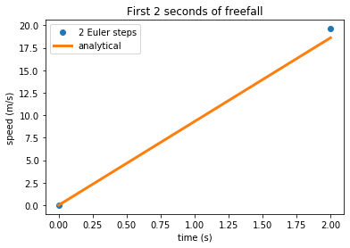
First, we solve for n=2 steps, so t=[0,2]. We can time the solution to get a sense of how long the computation will take for larger values of n.
%%time
n=2

v_analytical,v_numerical,t=freefall(n);
CPU times: user 288 µs, sys: 3 µs, total: 291 µs
Wall time: 303 µs
The block of code above assigned three variables from the function freefall.
v_analytical= \(v_{terminal}\tanh{\left(\frac{gt}{v_{terminal}}\right)}\)v_numerical= Euler step integration of \(\frac{dv}{dt}= g - \frac{c}{m}v^2\)t= timesteps from 0..2 withnvalues, here t=np.array([0,2])
All three variables have the same length, so we can plot them and visually compare v_analytical and v_numerical. This is the comparison method (1) from above.
import matplotlib.pyplot as plt
%matplotlib inline
plt.plot(t,v_numerical,'o',label=str(n)+' Euler steps')
plt.plot(t,v_analytical,label='analytical')
plt.title('First 2 seconds of freefall')
plt.xlabel('time (s)')
plt.ylabel('speed (m/s)')
plt.legend()
<matplotlib.legend.Legend at 0x7f131d486c90>
Exercise
Try adjusting n in the code above to watch the solution converge. You should notice the Euler approximation becomes almost indistinguishable from the analytical solution as n increases.
Convergence of a numerical model
You should see that the more time steps we use, the closer the Euler approximation resembles the analytical solution. This is true only to a point, due to roundoff error. In our freefall function, the numerical result is saved as a 32-bit floating point array. Our best approximation of the freefall function is the 64-bit analytical equation v_terminal*np.tanh(g*t/v_terminal).\(^{+}\)
In the next plot, we consider the relative error for the velocity at t=2 s, as a function of N.
\(^+\) Note: In practice, there is no reason to restrict the precision of our floating point numbers. The function was written this way to highlight the effect of roundoff error without significant computational resources. You would need significantly more timesteps to observe floating point error with 64-bit floating point numbers.
N=100
error=np.zeros(N)    # initialize an N-valued array of relative errors
n=np.logspace(2,5,N) # create an array from 10^2 to 10^5 with N values
for i in range(0,N):
    v_an,v_num,t=freefall(n[i]) # return the analytical and numerical solutions to our equation
    error[i]=(v_num[-1]-v_an[-1])/v_an[-1] #calculate relative error in velocity at final time t=2 s
plt.loglog(n,error,'o')
plt.xlabel('number of timesteps N')
plt.ylabel('relative error')
plt.title('Truncation and roundoff error \naccumulation in log-log plot')
Text(0.5, 1.0, 'Truncation and roundoff error \naccumulation in log-log plot')
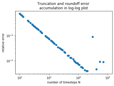
In the above plot “Truncation and roundoff error accumulation in log-log plot”, we see that around N=20,000 steps we stop decreasing the error with more steps. This is because we are approaching the limit of how precise we can store a number using a 32-bit floating point number.
In any computational solution, there will be some point of similar diminishing in terms of accuracy (error) and computational time (in this case, number of timesteps). If you were to attempt a solution for N=1 billion, the solution could take \(\approx\)(1 billion)*(200 \(\mu\)s[cpu time for n=2])\(\approx\)55 hours, but would not increase the accuracy of the solution.
What we’ve learned
Numerical integration with the Euler approximation
The source of truncation errors
The source of roundoff errors
How to time a numerical solution or a function
How to compare solutions
The definition of absolute error and relative error
How a numerical solution converges
Problems
The growth of populations of organisms has many engineering and scientific applications. One of the simplest models assumes that the rate of change of the population p is proportional to the existing population at any time t:
\(\frac{dp}{dt} = k_g p\)
where \(t\) is time in years, and \(k_g\) is growth rate in [1/years].
The world population has been increasing dramatically, let’s make a prediction based upon the following data saved in world_population_1900-2020.csv:
year
world population
1900
1,578,000,000
1950
2,526,000,000
2000
6,127,000,000
2020
7,795,482,000
a. Calculate the average population growth, \(\frac{\Delta p}{\Delta t}\), from 1900-1950, 1950-2000, and 2000-2020
b. Determine the average growth rates. \(k_g\), from 1900-1950, 1950-2000, and 2000-2020
c. Use a growth rate of \(k_g=0.013\) [1/years] and compare the analytical solution (use initial condition p(1900) = 1578000000) to the Euler integration for time steps of 20 years from 1900 to 2020 (Hint: use method (1)- plot the two solutions together with the given data)
d. Discussion question: If you decrease the time steps further and the solution converges, will it converge to the actual world population? Why or why not?
Note: We have used a new function np.loadtxt here. Use the help or ? to learn about what this function does and how the arguments can change the output. In the next module, we will go into more details on how to load data, plot data, and present trends.
import numpy as np
year,pop=np.loadtxt('./data/world_population_1900-2020.csv',skiprows=1,delimiter=',',unpack=True)
print('years=',year)
print('population =', pop)
years= [1900. 1950. 2000. 2020.]
population = [1.578000e+09 2.526000e+09 6.127000e+09 7.795482e+09]
dpdt = (pop[1:]-pop[0:-1])/(year[1:]-year[0:-1])
print('population changes in millions of people/year\n1900: {}\n1950: {}\n2000: {}'.format(*dpdt/1e6))
population changes in millions of people/year
1900: 18.96
1950: 72.02
2000: 83.4241
print('population growth rate in 1/years \n1900: {}\n1950: {}\n2000: {}'.format(*dpdt/pop[0:-1]))
population growth rate in 1/years
1900: 0.012015209125475285
1950: 0.028511480601741884
2000: 0.013615815244001959
p = lambda t: pop[0]*np.exp(0.013*(t-year[0]))
t=np.linspace(1900,2030,30)
dt=t[1]-t[0]
plt.plot(t,p(t),label='analytical')
p_euler = np.zeros(len(t))
p_euler[0] = pop[0]
for i in range(0,len(t)-1):
    p_euler[i+1]= p_euler[i]+0.013*p_euler[i]*dt

plt.plot(t,p_euler,'-.',label='euler {} steps'.format(len(t)))

t=np.linspace(1900,2030,100)
dt=t[1]-t[0]
p_euler = np.zeros(len(t))
p_euler[0] = pop[0]
for i in range(0,len(t)-1):
    p_euler[i+1]= p_euler[i]+0.013*p_euler[i]*dt
plt.plot(t,p_euler,'--',label='euler {} steps'.format(len(t)))

plt.plot(year,pop,'s',label='measured populations')
plt.legend();
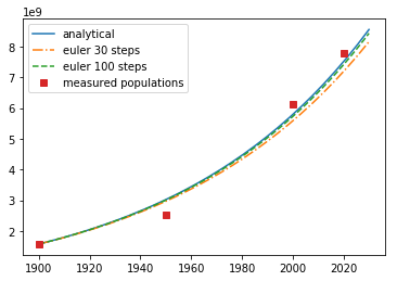
d. As the number of time steps increases, the Euler approximation approaches the analytical solution, not the measured data. The best-case scenario is that the Euler solution is the same as the analytical solution.
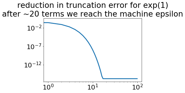
In the freefall example we used smaller time steps to decrease the truncation error in our Euler approximation. Another way to decrease approximation error is to continue expanding the Taylor series. Consider the function f(x)
\(f(x)=e^x = 1+x+\frac{x^2}{2!}+\frac{x^3}{3!}+\frac{x^4}{4!}+...\)
We can approximate \(e^x\) as \(1+x\) (first order), \(1+x+x^2/2\) (second order), and so on each higher order results in smaller error.
a. Use the given
exptaylorfunction to approximate the value of exp(1) with a second-order Taylor series expansion. What is the relative error compared tonp.exp(1)?b. Time the solution for a second-order Taylor series and a tenth-order Taylor series. How long would a 100,000-order series take (approximate this, you don’t have to run it)
c. Plot the relative error as a function of the Taylor series expansion order from first order upwards. (Hint: use method (4) in the comparison methods from the “Truncation and roundoff error accumulation in log-log plot” figure)
from math import factorial
def exptaylor(x,n):
    '''Taylor series expansion about x=0 for the function e^x
    the full expansion follows the function
    e^x = 1+ x + x**2/2! + x**3/3! + x**4/4! + x**5/5! +...'''
    if n<1:
        print('lowest order expansion is 0 where e^x = 1')
        return 1
    else:
        ex = 1+x # define the first-order taylor series result
        for i in range(1,n):
            ex+=x**(i+1)/factorial(i+1) # add the nth-order result for each step in loop
        return ex
n=np.arange(0,100)
error = np.zeros(len(n))
exp1 = np.exp(1)
for i in range(len(n)):
    e1=exptaylor(1,n[i])
    error[i] = np.abs(e1-exp1)/exp1
plt.loglog(n,error)
plt.title('reduction in truncation error for exp(1)\nafter ~20 terms we reach the machine epsilon');
lowest order expansion is 0 where e^x = 1