Homework #4
Contents
import numpy as np
from numpy import sin,cos,pi
import matplotlib.pyplot as plt
plt.style.use('fivethirtyeight')
Homework #4
Problem 1
The pendulum bob of mass m, shown in the figure above, is suspended by an inextensible string from the point p. This point is free to move along a straight horizontal line under the action of the springs, each having a constant k. Assume that the mass is displaced only slightly from the equilibrium position and released. Neglecting the mass of the springs, show that the pendulum oscillates with a period of
\(P=2\pi\sqrt{\frac{mg+2kr}{2kg}}\)
use a first-order Taylor series approximation for \(\sin\theta\approx\theta\) and \(\cos\theta\approx 1\)
Solve for \(\theta(t)\) if m=0.1 kg, r=1 m, \(\theta(0)\)=pi/6 rad, and \(\dot{\theta}(0)\)=0 rad/s for 2 cases:
a. k=20 N/m
b. k=\(\infty\) N/m
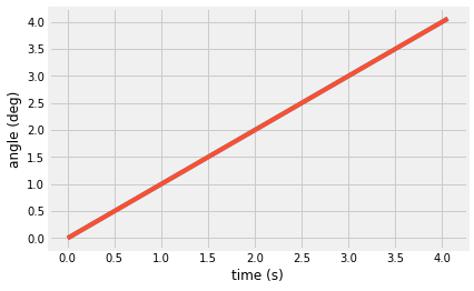
c. Plot the solutions of \(\theta(t)\) for 2 periods on one figure
l=1
m=0.1
k=20
g=9.81
P=2*pi/np.sqrt(2*k*g/(2*k*l+m*g))

t=np.linspace(0,2*P);
# your work
# your new solutions, convert rad to deg with 180/pi
a_inf = t # create solution for k=infty
a_20 = t # create solution for k=20 N/m

plt.plot(t,a_inf)
plt.plot(t,a_20)
plt.xlabel('time (s)')
plt.ylabel('angle (deg)')
Text(0, 0.5, 'angle (deg)')

from scipy.linalg import *
from scipy.optimize import fsolve,root
from scipy.integrate import solve_ivp # import the ordinary differential equation integrator in Python
Problem 2
from IPython.display import YouTubeVideo
YouTubeVideo('eOvwiYRroso')
The pendulum arm of mass m, shown in the figure above, is held in place by two springs. This point is free to move along a straight horizontal line under
the action of the springs, each having a constant k. Assume that the mass is displaced
only slightly from the equilibrium position and released. Neglecting the mass of the
springs, solve for the nonlinear equations of motion and use the solve_ivp to determine \(\theta(t)\)
Solve for \(\theta(t)\) if m=1 kg, L=1 m, \(\theta(0)\)=pi/6 rad, and \(\dot{\theta}(0)\)=0 rad/s for
k=20 N/m
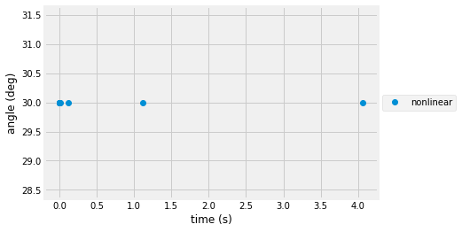
Plot the nonlinear solutions of \(\theta(t)\) for 2 periods on one figure
def my_ode(t,r,):
    """ Help documentation for "my_ode"
     input is time, t (s) and r=[position p (m), angle (rad), velocity p (m/s), angle velocity (rad/s)] and time
     output is dr=[velocity p (m/s), angle velocity (rad/s), accel p (m/s/s), angle accel (rad/s/s)] at time, t
     the ODE is defined by:

     dr = f(t,r)"""
    l=1
    m=0.1
    k=20
    g=9.81
    dr=np.zeros(np.size(r))
    dr[0]=r[2]
    dr[1]=r[3]
    # your work here
    # dr[2] =...
    # dr[3] =...
    return dr
P=2*pi/np.sqrt(2*k*g/(2*k*l+m*g))
r=solve_ivp(my_ode,[0,2*P],[0, pi/6,0,0]); # default = 'RK45'
plt.plot(r.t,r.y[1]*180/pi,'o',label='nonlinear') # <-------------- your new plot, convert rad to deg with 180/pi
plt.legend(loc='center left', bbox_to_anchor=(1, 0.5))
plt.xlabel('time (s)')
plt.ylabel('angle (deg)')
Text(0, 0.5, 'angle (deg)')

