Solving the equations of motion for a spinning top
Contents
import numpy as np
from numpy import sin, cos, pi
from scipy.integrate import solve_ivp
import matplotlib.pyplot as plt
plt.style.use('fivethirtyeight')
Solving the equations of motion for a spinning top
In this notebook, you will use the differential equations of motion for a spinning top. You will
create a function that returns the derivative of the state in the form \(\dot{\mathbf{y}} = f(\mathbf{y})\)
use
solve_ivpto integrate the initial value problemcompare the solution to the predicted result \(\dot{\phi} = \frac{mgd}{I_z\dot{\psi}}\)
Background and setup
In this lecture video, you choose 3 generalized coordinates, then determine 3 coupled differential equations for a top that is spinning on a fixed origin. The generalized coordinates represent 3 types of motion for the spinning top:
\(\psi\) - spin angle (how much the top has rotated)
\(\phi\) - precession (the rotation of the whole system around the fixed point)
\(\theta\) - nutate (the angle that the top is rotated away from vertical)
The position of the top’s center of mass is
\(\mathbf{r}_{G} = x\hat{i} + y\hat{j} +z \hat{k}\)
where
\(x = d\sin(\theta)\cos(\phi)\)
\(y = d\sin(\theta)\sin(\phi)\)
\(z = d\cos(\theta)\)
The Lagrangian for the spinning top is as follows:
\(L = T-V= \frac{1}{2}\mathbf{\omega I_O\omega} - mgz\)
where
\(\mathbf{\omega} = \dot{\theta}\hat{i}' + \dot{\phi}\sin\theta\hat{j}' + (\dot{\phi}\cos\theta +\dot{\psi})\hat{k}'\)
\(\mathbf{I_O} = \left[\begin{array} ~I_x +md^2 & 0 & 0\\ 0 & I_y +md^2 & 0\\ 0 & 0 & I_z \end{array}\right]\)
assuming \(I_x=I_y\), then \(I_O = I_x +md^2\)
Equations of motion
General equations
Leading to two first-order differential equations that describe conservation of angular momentum and one second order differential equation as such
\(\frac{\partial L}{\partial \dot{\phi}} = \dot{\phi}(I_O\sin^2\theta+I_z\cos^2\theta) +I_z\dot{\psi}\cos\theta = cst = p_\phi\)
\(\frac{\partial L}{\partial \dot{\psi}} = I_z(\dot{\psi}+\dot{\phi}\cos\theta) = cst = p_\psi\)
\(I_O\ddot{\theta} - \dot{\phi}^2\sin\theta\cos\theta(I_O-I_z)+\dot{\phi}\dot{\psi}I_z\sin\theta-mgd\sin\theta = 0\)

Consider a slender support, connected to a spinning disk where
\(m=0.1~kg\)
\(r=0.1~m\)
\(d = 2r = 0.2~m\)
m = 0.1
r = 0.1
d = 2*r
def top_ode(t, y, spin=500, theta0=pi/6, d = d):
    '''

    top_ode(t, y, spin, theta0, d):

    Return the derivative for a spinning top fixed to the origin with center of
    mass at distance, `d`, from the origin

    Parameters
    ----------
    t: current time
    y: current state = y = [phi, psi, theta, dtheta/dt]
    spin: initial spin rate (optional) default is 500 rad/s
    theta0: initial nutation angle (optional) default is 30 deg, pi/6
    d: distance from origin to center of mass (optional) default uses defined d value

    Returns
    -------
    dy: derivative of state, y, at time, t
        [dphi/dt, dpsi/dt, dtheta/dt, ddtheta/ddt]
    '''
    Io = 1/4*m*r**2+m*d**2
    Iz = 1/2*m*r**2
    dy = np.zeros(y.shape)

    Pphi = Iz*spin*cos(theta0)
    Ppsi = Iz*spin

    DP = (Io*sin(y[2])**2+Iz*cos(y[2])**2)*Iz - Iz**2*cos(y[2])**2

    if spin>0.001:
        # if the rate of spin is ~0, then the conservation of angular momentum
        # equations will be singular and should be replaced by 0's
        dy[0] = (Iz*Pphi - Iz*cos(y[2])*Ppsi)/DP
        dy[1] = (-Iz*cos(y[2])*Pphi + (Io*sin(y[2])**2+Iz*cos(y[2])**2)*Ppsi)/DP

    dy[2] = y[3]
    dy[3] = dy[0]**2*sin(y[2])*cos(y[2])*(Io-Iz)-\
            dy[0]*dy[1]*Iz*sin(y[2])+\
            m*9.81*d*sin(y[2])
    dy[3] = dy[3]/Io

    return dy
Precession for high spinning rate
In equation (3), if \(\dot{\psi}>>\dot{\theta},~\dot{\phi},~\ddot{\theta}\), then the equations simplify to one relationship between \(\dot{\psi}~and~\dot{\phi}\), spin and precession, respectively.
\(\dot{\phi} = \frac{mgd}{I_z\dot{\psi}}~\frac{rad}{s}\)
You will use the precession time period, \(T_{precess} = \frac{2\pi}{\dot{\phi}}~s\) as the solution interval, [0, T].
Io = 1/4*m*r**2+m*d**2
Iz = 1/2*m*r**2
spin = 500
Iz = 1/2*m*r**2
phi = m*9.81*d/Iz/spin
print('phi = {:.3f} rad/s'.format(phi))
print('phi = {:.3f} cycles/s'.format(phi/2/pi))
print('precession time period {:.2f}'.format(2*pi/phi), ' s')
phi = 0.785 rad/s
phi = 0.125 cycles/s
precession time period 8.01  s
Solve for the state over time
Here, you use the solve_ivp integration to solve for the state as a function of time,
\(state = [\phi,~\psi,~\theta,~\dot{\theta}]\) over time, \(t=\left[0...\frac{2\pi}{\dot{\phi}}\right]\)
spin = 500
theta0 = pi/6
T = 2*pi*Iz*spin/(m*9.81*d)
sol = solve_ivp(lambda t, y: top_ode(t,y, spin = spin, theta0 = theta0),
                [0,T],
                np.array([0, 0, theta0, 0]),
                t_eval=np.linspace(0,T,1000))
Verify solution
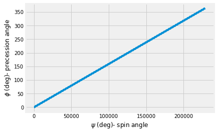
Here, you expect the result that \(\dot{\phi}\dot{\psi}=cst\). So, if you plot \(\phi(t)-vs-\psi(t)\), you should see a straight line if \(\dot{\psi}\) is very large.
plt.plot(sol.y[1]*180/pi, sol.y[0]*180/pi)
plt.xlabel(r'$\psi$ (deg)- spin angle')
plt.ylabel(r'$\phi$ (deg)- precession angle');
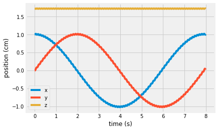
Look at position of top
Here, use the solution of the state variable, sol.y to plug into the kinematic equations for the position of the top over time. You should expect a cosine and sine for \(x(t)~and~y(t)\), respectively. The solution should plot one full period, since you used the time period of precession as the end time in solve_ivp.
x = d*sin(sol.y[2])*cos(sol.y[0])
y = d*sin(sol.y[2])*sin(sol.y[0])
z = d*cos(sol.y[2])
plt.plot(sol.t, 10*x, label = 'x')
plt.plot(sol.t, 10*y, label = 'y')
plt.plot(sol.t, 10*z, label = 'z')
plt.xlabel('time (s)')
plt.ylabel('position (cm)')
plt.legend();
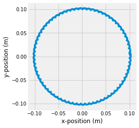
Animate the motion of the top
In the next code cells, you will set up a 2D animation to watch the top nutate and precess around the origin. You will plot the position of the center of mass for each point in time and plot a line for the path it has followed up until the current time.
from matplotlib import animation
from IPython.display import HTML
fig, ax = plt.subplots()
line, = ax.plot(x, y)
marker, = ax.plot([], [], '+', markersize=30)
S = x.max()*1.1
ax.set(xlim=(-S, S))
ax.set_aspect('equal')
ax.set_xlabel('x-position (m)')
ax.set_ylabel('y-position (m)');
Create an initializing (
init) function that clears the previous line and marker
def init():
    line.set_data([], [])
    marker.set_data([], [])
    return (line,marker,)
Create an animating (
animate) function that updates the line
def animate(i):
    '''function that updates the line and marker data
    arguments:
    ----------
    i: index of timestep
    outputs:
    --------
    line: the line object plotted in the above ax.plot(...)
    marker: the marker for the end of the 2-bar linkage plotted above with ax.plot('...','o')'''
    line.set_data(x[:i], y[:i])
    marker.set_data(x[i], y[i])
    return (line, marker, )
Create an animation (
anim) variable using theanimation.FuncAnimation
anim = animation.FuncAnimation(fig, animate, init_func=init,
                               frames=range(0,len(x)), interval=10,
                               blit=True)
HTML(anim.to_html5_video())
Wrapping up
In this notebook, you solved for the position of a spinning top by considering
spin, \(\dot{\psi}\)
precession, \(\dot{\phi}\)
nutation, \(\dot{\theta}\)
You compared approximate solutions for two cases when the top is spinning fast:
analytical approximation using a limit
numerical integration of the exact differential equations