Rotating Pendulum solution - integrating equation of motion¶

Creating equation of motion for rotating pendulum

Setup¶

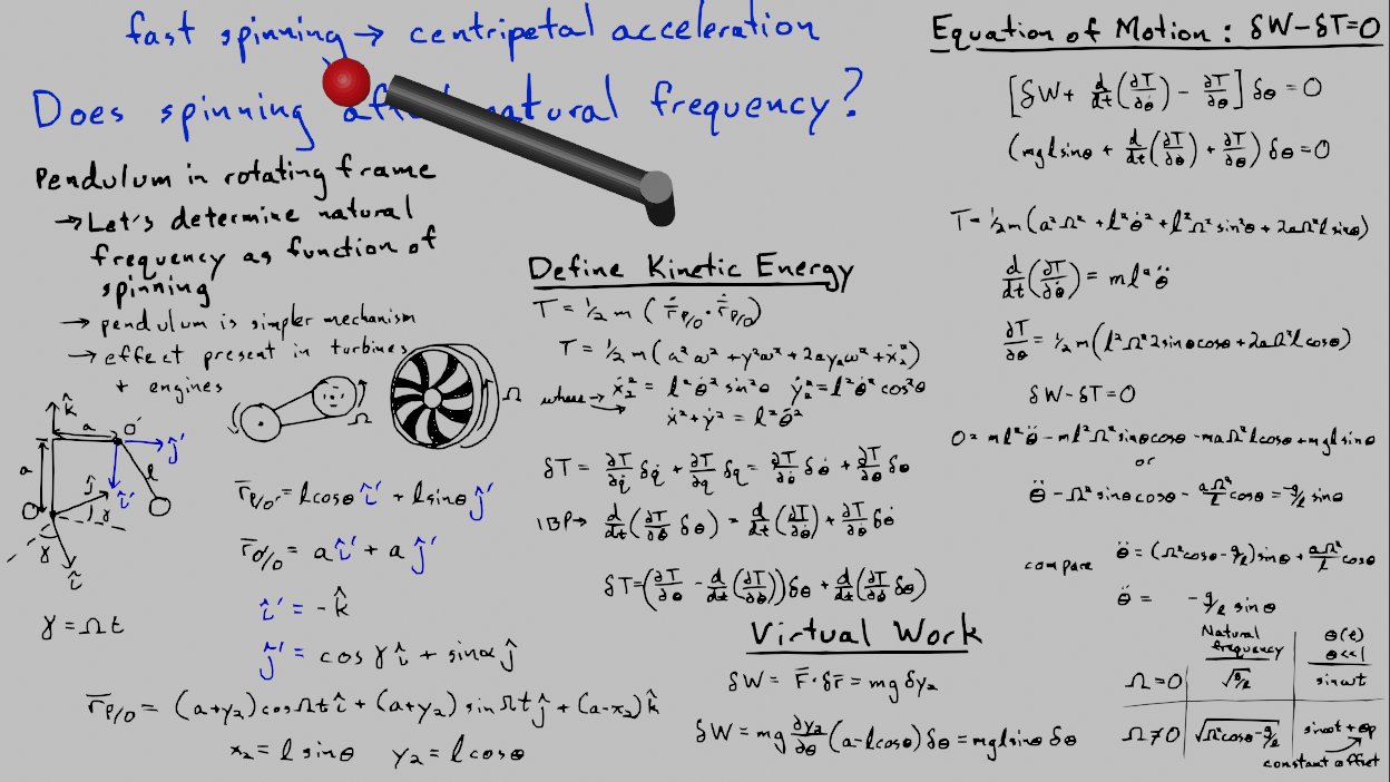
In this lecture you solve for the the natural frequency of a pendulum in a rotating reference frame. The result is an equation of motion as such

\(\ddot{\theta} = \left(\Omega^2\cos\theta -\frac{g}{l}\right)\sin\theta +\frac{a\Omega^2}{l}\cos\theta\)

where \(\Omega\) is the rotation rate of the frame holding the pendulum, \(a\) is the distance from the point of rotation, \(l\) is the pendulum length, and \(\theta\) is the generalized coordinate that describes the pendulum’s position in the rotating reference frame.

Consider the cases

case	natural frequency	function \(\theta(t)\) for \(\theta<<1\)
\(\Omega = 0\)	\(\omega = \sqrt{\frac{g}{l}}\)	\(\theta(t) = \sin\omega t\)
\(\Omega \neq 0\)	\(\omega = \sqrt{\frac{g}{l}-\Omega^2\cos\theta}\)	\(\theta(t) = \sin\omega t+\theta_{offset}\)

These solutions only account for small angles, if \(\Omega^2\cos\theta>\frac{g}{l}\), the natural frequency becomes imaginary and the solution is an exponential growth, assuming \(\sin\theta=\theta\). The actual solution, shouldn’t have an angular speed that keeps growing.

Building a numerical solution¶

Instead of using differential equations to solve for \(\theta(t)\), you can use scipy.integrate.solve_ivp to create a numerical solution to the differential equation.

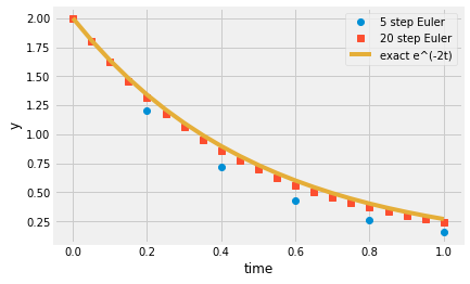
A numerical solution does not return a mathematical function. Instead, it returns the predicted solution based upon the differential equations. The simplest numerical solution is the Euler integration. Consider an exponential decay ODE,

\(\frac{dy}{dt} = -2y\)

The exact solution is \(y(t) = y_0e^{-2t}\), but you can approximate this solution without doing any calculus. Make the approximation

\(\frac{\Delta y}{\Delta t} = -2y\)

Now, you have an algebraic equation,

\(\frac{y_{i+1}-y_{i}}{\Delta t} = -2y_i\)

where \(\Delta t\) is a chosen timestep the smaller the better, \(y_i\) is the current value of \(y\), and \(y_{i+1}\) is the approximated next value of \(y\). Consider the initial condition \(y(0)=2\) and take a time step of \(\Delta t =0.1\)

\(y_{i+1} = y_{i}-2y_{i}\Delta t\)

\(y(\Delta t) = 2 - 2(0.1) = 1.8\)

The exact solution is \(y(0.1) = 1.637\), you can make more exact solutions with smaller steps as seen below.

t = np.linspace(0, 1, 6)
dt = t[1] - t[0]
ynum = np.zeros(t.shape)
ynum[0] = 2
for i in range(1,len(t)):
    ynum[i] = ynum[i-1]-2*ynum[i-1]*dt

plt.plot(t, ynum, 'o', label = '5 step Euler')

t = np.linspace(0, 1, 21)
dt = t[1] - t[0]
ynum = np.zeros(t.shape)
ynum[0] = 2
for i in range(1,len(t)):
    ynum[i] = ynum[i-1]-2*ynum[i-1]*dt

plt.plot(t, ynum, 's', label = '20 step Euler')

plt.plot(t, 2*np.exp(-2*t), label = 'exact e^(-2t)')
plt.legend()
plt.xlabel('time')
plt.ylabel('y')

Text(0, 0.5, 'y')

Define ODE for rotating pendulum¶

Numerical integration requires first-order differential equations, but here you have a second-order differential equation. You can rewrite your single second-order equation of motion as two first-order equations of motion as such

\(\bar{y} = [\theta,~\dot{\theta}]\)

\(\dot{\bar{y}} = [\dot{\theta},~\ddot{\theta}]\)

\(\ddot{\theta} = f(t,\theta, \dot{\theta})\rightarrow \dot{\bar{y}} = f(t,~\bar{y})\)

take a look at the function defining the derived equation of motion, pend_rot(t, y)

first output is taken from the input, dy[0] = y[1]: \(\frac{d}{dt}\theta = \dot{\theta}\)
the second output is taken from the equation of motion directly, dy[1]= \(\ddot{\theta} = \left(\Omega^2\cos\theta -\frac{g}{l}\right)\sin\theta +\frac{a\Omega^2}{l}\cos\theta\)

def pend_rot(t, y, w, l = 0.3, a = 1):
    '''
    function that defines 2 first-order ODEs for a rotating pendulum
    arguments:
    ----------
    t: current time
    y: current angle and angular velocity of pendulum [theta (rad), dtheta(rad/s)]
    w: rotation rate of frame in (rad/s)
    l: length of pendulum arm
    a: distance from point of rotation
    
    outputs:
    --------
    dy: derivative of y at time t [dtheta (rad/s), ddtheta(rad/s/s)] 
    '''
    dy=np.zeros(y.shape)
    dy[0]=y[1]
    dy[1]=(w**2*np.cos(y[0])-9.81/l)*np.sin(y[0])+a*w**2/l*np.cos(y[0])
    return dy

Solving the equation of motion¶

Now that you have defined pend_rot, you can import solve_ivp and solve for \(\theta\) as a function of time.

Import scipy.integrate.solve_ivp

from scipy.integrate import solve_ivp

plug in values for the constants and solve for one full cycle at \(\Omega=1~rad/s\) i.e. \(1~cycle\frac{2\pi~rad}{cycle}\frac{1~rad}{s}\)

l=0.3
a=1
w=1
g=9.81
T = 2*np.pi
my_ode = lambda t,y: pend_rot(t,y,w = w, l = l, a = a)

sol = solve_ivp(my_ode,[0,T] , [np.pi/6,0], 
                t_eval = np.linspace(0,T,600));

Your results are now saved in the variable sol:

sol.t: array of points in time where the integration returned a solution
sol.y: array of two values (sol.y[0] = \(\theta(t)\) and sol.y[1] = \(\dot{\theta}(t))\)

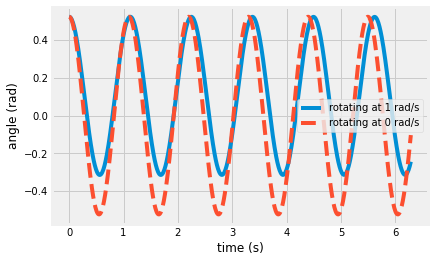
Plot the result to compare to a hanging pendulum. You used an initial resting state with \(\theta(0) = \frac{\pi}{12}\). The non-rotating solution is

\(\theta(t) = \frac{\pi}{6}\cos\sqrt{\frac{g}{l}} t\)

plt.plot(sol.t,sol.y[0,:], label = 'rotating at {} rad/s'.format(w))
plt.plot(sol.t, np.pi/6*np.cos(np.sqrt(g/l)*sol.t),'--', label = 'rotating at 0 rad/s')

plt.legend()
plt.xlabel('time (s)')
plt.ylabel('angle (rad)');

Visualize the motion with animations¶

This is great, but what does the motion look like? Now, use the kinematic definitions to define 3D coordinates of the frame and pendulum arm.

\(r_{P/O} = (a+y_2)\cos(\Omega t) \hat{i} +(a+y_2)\sin\Omega t \hat{j} +(a-x_2)\hat{k} = x_1\hat{i} +y_1\hat{j}+z_1 \hat{k}\)
\(x_2= l\sin\theta\)
\(y_2= l\cos\theta\)
link arm goes from \((0,~0,~0) \rightarrow (0,~0,~a) \rightarrow (a\cos\Omega t, a\sin\Omega t, a)\)

t = sol.t
y = sol.y
x1=np.cos(w*t)*(a+l*np.sin(y[0,:])) # x1-coordinate over time
y1=np.sin(w*t)*(a+l*np.sin(y[0,:])) # y1-coordinate over time
z1=a-l*np.cos(y[0,:]);          # z1-coordinate over time
linkx=np.block([np.zeros((len(t),1)), 
               np.zeros((len(t),1)), 
               a*np.cos(w*t[:,np.newaxis])])
linky=np.block([np.zeros((len(t),1)), 
                np.zeros((len(t),1)), 
                a*np.sin(w*t[:,np.newaxis])])
linkz=np.block([np.zeros((len(t),1)), 
                a*np.ones((len(t),1)), 
                a*np.ones((len(t),1))])

The kinematics are now defined for the pendulum and frame in the fixed, 3D coordinate system. You can import animation and plot the frame and pendulum.

from matplotlib import animation
from IPython.display import HTML

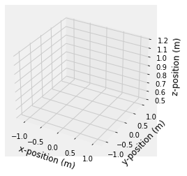
Here, you set up the 3D axes for plotting and the line updating functions, init and animate.

fig = plt.figure()
ax = fig.add_subplot(111, projection='3d')
line1, = ax.plot([], [], [])
line2, = ax.plot([], [], [], 'o-')
line3, = ax.plot([], [], [], '--')
ax.set_xlim(-1.2,1.2)
ax.set_ylim(-1.2,1.2)
ax.set_zlim(0.5,1.2)

#ax.view_init(elev=10., azim=10)
ax.set_xlabel('x-position (m)')
ax.set_ylabel('y-position (m)')
ax.set_zlabel('z-position (m)')

def init():
    line1.set_data([], [])
    line1.set_3d_properties([])
    line2.set_data([], [])
    line2.set_3d_properties([])
    line3.set_data([], [])
    line3.set_3d_properties([])
    return (line1, line2, line3)

def animate(i):
    line1.set_data(linkx[i,:], linky[i,:])
    line1.set_3d_properties(linkz[i,:])
    line2.set_data([linkx[i,2], x1[i]], [linky[i,2], y1[i]])
    line2.set_3d_properties([linkz[i,2], z1[i]])
    line3.set_data(x1[:i], y1[:i])
    line3.set_3d_properties(z1[:i])
    return (line1, line2, line3, )

Now, animate the motion of the pendulum and its path.

anim = animation.FuncAnimation(fig, animate, init_func=init,
                               frames=range(0,len(t)), interval=10, 
                               blit=True)

HTML(anim.to_html5_video())

Wrapping up¶

In this notebook, you created a general solution for nonlinear differential equations. You did this by:

creating 2 first-order differential equations from one second-order differential equation
defining a function that returns the derivative based upon the current state \((\theta,~\dot{\theta})\)
using solve_ivp to integrate the differential equations

Once you had a solution, you processed the results by:

plotting the generalized coordinate vs time
comparing the solution to a known result
plugging the generalized coordinate into the defining kinematics
creating a 3D animation of your solution

Nice work!

Advanced Dynamics

Rotating Pendulum solution - integrating equation of motion

Contents