CompMech04-Linear Algebra Project#
Practical Linear Algebra for Finite Element Analysis#
In this project we will perform a linear-elastic finite element analysis (FEA) on a support structure made of 11 beams that are riveted in 7 locations to create a truss as shown in the image below.
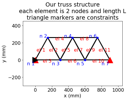
The triangular truss shown above can be modeled using a direct stiffness method [1], that is detailed in the extra-FEA_material notebook. The end result of converting this structure to a FE model. Is that each joint, labeled \(n~1-7\), short for node 1-7 can move in the x- and y-directions, but causes a force modeled with Hooke’s law. Each beam labeled \(el~1-11\), short for element 1-11, contributes to the stiffness of the structure. We have 14 equations where the sum of the components of forces = 0, represented by the equation
\(\mathbf{F-Ku}=\mathbf{0}\)
Where, \(\mathbf{F}\) are externally applied forces, \(\mathbf{u}\) are x- and y- displacements of nodes, and \(\mathbf{K}\) is the stiffness matrix given in fea_arrays.npz as K, shown below
note: the array shown is 1000x(K). You can use units of MPa (N/mm^2), N, and mm. The array K is in 1/mm
\(\mathbf{K}=EA*\)
\( \left[ \begin{array}{cccccccccccccc} 4.2 & 1.4 & -0.8 & -1.4 & -3.3 & 0.0 & 0.0 & 0.0 & 0.0 & 0.0 & 0.0 & 0.0 & 0.0 & 0.0 \\ 1.4 & 2.5 & -1.4 & -2.5 & 0.0 & 0.0 & 0.0 & 0.0 & 0.0 & 0.0 & 0.0 & 0.0 & 0.0 & 0.0 \\ -0.8 & -1.4 & 5.0 & 0.0 & -0.8 & 1.4 & -3.3 & 0.0 & 0.0 & 0.0 & 0.0 & 0.0 & 0.0 & 0.0 \\ -1.4 & -2.5 & 0.0 & 5.0 & 1.4 & -2.5 & 0.0 & 0.0 & 0.0 & 0.0 & 0.0 & 0.0 & 0.0 & 0.0 \\ -3.3 & 0.0 & -0.8 & 1.4 & 8.3 & 0.0 & -0.8 & -1.4 & -3.3 & 0.0 & 0.0 & 0.0 & 0.0 & 0.0 \\ 0.0 & 0.0 & 1.4 & -2.5 & 0.0 & 5.0 & -1.4 & -2.5 & 0.0 & 0.0 & 0.0 & 0.0 & 0.0 & 0.0 \\ 0.0 & 0.0 & -3.3 & 0.0 & -0.8 & -1.4 & 8.3 & 0.0 & -0.8 & 1.4 & -3.3 & 0.0 & 0.0 & 0.0 \\ 0.0 & 0.0 & 0.0 & 0.0 & -1.4 & -2.5 & 0.0 & 5.0 & 1.4 & -2.5 & 0.0 & 0.0 & 0.0 & 0.0 \\ 0.0 & 0.0 & 0.0 & 0.0 & -3.3 & 0.0 & -0.8 & 1.4 & 8.3 & 0.0 & -0.8 & -1.4 & -3.3 & 0.0 \\ 0.0 & 0.0 & 0.0 & 0.0 & 0.0 & 0.0 & 1.4 & -2.5 & 0.0 & 5.0 & -1.4 & -2.5 & 0.0 & 0.0 \\ 0.0 & 0.0 & 0.0 & 0.0 & 0.0 & 0.0 & -3.3 & 0.0 & -0.8 & -1.4 & 5.0 & 0.0 & -0.8 & 1.4 \\ 0.0 & 0.0 & 0.0 & 0.0 & 0.0 & 0.0 & 0.0 & 0.0 & -1.4 & -2.5 & 0.0 & 5.0 & 1.4 & -2.5 \\ 0.0 & 0.0 & 0.0 & 0.0 & 0.0 & 0.0 & 0.0 & 0.0 & -3.3 & 0.0 & -0.8 & 1.4 & 4.2 & -1.4 \\ 0.0 & 0.0 & 0.0 & 0.0 & 0.0 & 0.0 & 0.0 & 0.0 & 0.0 & 0.0 & 1.4 & -2.5 & -1.4 & 2.5 \\ \end{array}\right]~\frac{1}{m}\)
import numpy as np
import matplotlib.pyplot as plt
plt.style.use('fivethirtyeight')
fea_arrays = np.load('./fea_arrays.npz')
K=fea_arrays['K']
K
array([[ 0.00416667,  0.00144338, -0.00083333, -0.00144338, -0.00333333,
         0.        ,  0.        ,  0.        ,  0.        ,  0.        ,
         0.        ,  0.        ,  0.        ,  0.        ],
       [ 0.00144338,  0.0025    , -0.00144338, -0.0025    ,  0.        ,
         0.        ,  0.        ,  0.        ,  0.        ,  0.        ,
         0.        ,  0.        ,  0.        ,  0.        ],
       [-0.00083333, -0.00144338,  0.005     ,  0.        , -0.00083333,
         0.00144338, -0.00333333,  0.        ,  0.        ,  0.        ,
         0.        ,  0.        ,  0.        ,  0.        ],
       [-0.00144338, -0.0025    ,  0.        ,  0.005     ,  0.00144338,
        -0.0025    ,  0.        ,  0.        ,  0.        ,  0.        ,
         0.        ,  0.        ,  0.        ,  0.        ],
       [-0.00333333,  0.        , -0.00083333,  0.00144338,  0.00833333,
         0.        , -0.00083333, -0.00144338, -0.00333333,  0.        ,
         0.        ,  0.        ,  0.        ,  0.        ],
       [ 0.        ,  0.        ,  0.00144338, -0.0025    ,  0.        ,
         0.005     , -0.00144338, -0.0025    ,  0.        ,  0.        ,
         0.        ,  0.        ,  0.        ,  0.        ],
       [ 0.        ,  0.        , -0.00333333,  0.        , -0.00083333,
        -0.00144338,  0.00833333,  0.        , -0.00083333,  0.00144338,
        -0.00333333,  0.        ,  0.        ,  0.        ],
       [ 0.        ,  0.        ,  0.        ,  0.        , -0.00144338,
        -0.0025    ,  0.        ,  0.005     ,  0.00144338, -0.0025    ,
         0.        ,  0.        ,  0.        ,  0.        ],
       [ 0.        ,  0.        ,  0.        ,  0.        , -0.00333333,
         0.        , -0.00083333,  0.00144338,  0.00833333,  0.        ,
        -0.00083333, -0.00144338, -0.00333333,  0.        ],
       [ 0.        ,  0.        ,  0.        ,  0.        ,  0.        ,
         0.        ,  0.00144338, -0.0025    ,  0.        ,  0.005     ,
        -0.00144338, -0.0025    ,  0.        ,  0.        ],
       [ 0.        ,  0.        ,  0.        ,  0.        ,  0.        ,
         0.        , -0.00333333,  0.        , -0.00083333, -0.00144338,
         0.005     ,  0.        , -0.00083333,  0.00144338],
       [ 0.        ,  0.        ,  0.        ,  0.        ,  0.        ,
         0.        ,  0.        ,  0.        , -0.00144338, -0.0025    ,
         0.        ,  0.005     ,  0.00144338, -0.0025    ],
       [ 0.        ,  0.        ,  0.        ,  0.        ,  0.        ,
         0.        ,  0.        ,  0.        , -0.00333333,  0.        ,
        -0.00083333,  0.00144338,  0.00416667, -0.00144338],
       [ 0.        ,  0.        ,  0.        ,  0.        ,  0.        ,
         0.        ,  0.        ,  0.        ,  0.        ,  0.        ,
         0.00144338, -0.0025    , -0.00144338,  0.0025    ]])
In this project we are solving the problem, \(\mathbf{F}=\mathbf{Ku}\), where \(\mathbf{F}\) is measured in Newtons, \(\mathbf{K}\) =E*A*K is the stiffness in N/mm, E is Young’s modulus measured in MPa (N/mm^2), and A is the cross-sectional area of the beam measured in mm^2.
There are three constraints on the motion of the joints:
i. node 1 displacement in the x-direction is 0 = u[0]
ii. node 1 displacement in the y-direction is 0 = u[1]
iii. node 7 displacement in the y-direction is 0 = u[13]
We can satisfy these constraints by leaving out the first, second, and last rows and columns from our linear algebra description.
1. Calculate the condition of K and the condition of K[2:13,2:13].#
a. What error would you expect when you solve for u in K*u = F?
b. Why is the condition of K so large?
c. What error would you expect when you solve for u[2:13] in K[2:13,2:13]*u=F[2:13]
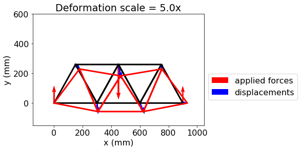
2. Apply a 300-N downward force to the central top node (n 4)#
a. Create the LU matrix for K[2:13,2:13]
b. Use cross-sectional area of \(0.1~mm^2\) and steel and almuminum moduli, \(E=200~GPa~and~E=70~GPa,\) respectively. Solve the forward and backward substitution methods for
\(\mathbf{Ly}=\mathbf{F}\frac{1}{EA}\)
\(\mathbf{Uu}=\mathbf{y}\)
your array F is zeros, except for F[5]=-300, to create a -300 N load at node 4.
c. Plug in the values for \(\mathbf{u}\) into the full equation, \(\mathbf{Ku}=\mathbf{F}\), to solve for the reaction forces
d. Create a plot of the undeformed and deformed structure with the
displacements and forces plotted as vectors (via quiver). Your result
for aluminum should match the following result from
extra-FEA_material. note: The scale factor is applied to displacements \(\mathbf{u}\), not forces.
Note: Look at the extra FEA material. It has example code that you can plug in here to make these plots. Including background information and the source code for this plot below.
3. Determine cross-sectional area#
a. Using aluminum, what is the minimum cross-sectional area to keep total y-deflections \(<0.2~mm\)?
b. Using steel, what is the minimum cross-sectional area to keep total y-deflections \(<0.2~mm\)?
c. What are the weights of the aluminum and steel trusses with the chosen cross-sectional areas?