Linear Regression Algebra

In the second Module CompMech02-Analyze-Data, you imported data from the NOAA (National Oceanic and Atmospheric Administration) youbpage. Then, you did a piece-wise linear regression fit, but the lines youre disconnected. In this notebook, you will look at general linear regression, which is framing the our least-sum-of-squares error as a linear algebra problem.

import numpy as np
import pandas as pd
import matplotlib.pyplot as plt
plt.style.use('fivethirtyeight')

Polynomials

In general, you may want to fit other polynomials besides degree-1 (straight-lines). You used the numpy.polyfit to accomplish this task before [1].

\(y=a_{0}+a_{1}x+a_{2}x^{2}+\cdots+a_{m}x^{m}+e\)

Now, the solution for \(a_{0},~a_{1},...a_{m}\) is the minimization of m+1-dependent linear equations.

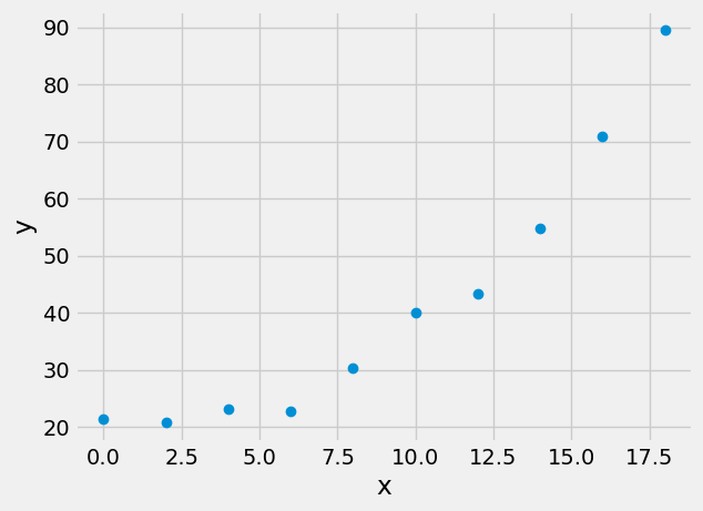
Consider the following data:

x	y
0.00	21.50
2.00	20.84
4.00	23.19
6.00	22.69
8.00	30.27
10.00	40.11
12.00	43.31
14.00	54.79
16.00	70.88
18.00	89.48

xy_data = np.loadtxt('../data/xy_data.csv',delimiter=',')
x=xy_data[:,0];
y=xy_data[:,1];
plt.plot(x,y,'o')
plt.xlabel('x')
plt.ylabel('y')

Text(0, 0.5, 'y')

A general polynomial decription of our function, \(f(\mathbf{x}),~and~\mathbf{y}\) is that you have \(m+1\) unknown coefficients, where \(m\) is the degree of the polynomial, and \(n\) independent equations. In the example framed below, you are choosing a second-order polnomial fit.

\(\mathbf{y}=\mathbf{x}^0 a_0+\mathbf{x}^1 a_1+\mathbf{x}^2 a_2+\mathbf{e}\)

\(\mathbf{y}=\left[\mathbf{Z}\right]\mathbf{a}+\mathbf{e}\)

where \(\mathbf{a}=\left[\begin{array}{c} a_{0}\\ a_{1}\\ a_{2}\end{array}\right]\)

\(\mathbf{y}=\left[\begin{array} 1y_{1} \\ y_{2} \\ y_{3} \\ y_{4} \\ y_{5} \\ y_{6} \\ y_{7} \\ y_{8} \\ y_{9} \\ y_{10} \end{array}\right]\) \(~~~~[\mathbf{Z}]=\left[\begin{array} 11 & x_{1} & x_{1}^{2} \\ 1 & x_{2} & x_{2}^{2} \\ 1 & x_{3} & x_{3}^{2} \\ 1 & x_{4} & x_{4}^{2} \\ 1 & x_{5} & x_{5}^{2} \\ 1 & x_{6} & x_{6}^{2} \\ 1 & x_{7} & x_{7}^{2} \\ 1 & x_{8} & x_{8}^{2} \\ 1 & x_{9} & x_{9}^{2} \\ 1 & x_{10} & x_{10}^{2} \end{array}\right]\)

The sum of squares residuals for this model is formed by solving for \(\mathbf{e}\), then summing the square of the elements

\(\mathbf{e} = \mathbf{y}-\mathbf{Za}\)

\(S_{r}=\sum_{i=1}^{n}\left(y_{i}-\sum_{j=0}^{m}a_{j}z_{ji}\right)^2\)

Minimizing this function, \(S_r\) results in the following set of linear equations,

\(\mathbf{y}=[\mathbf{Z}]\mathbf{a}\)

->A standard Linear Algebra Problem

the vector a is unknown, and Z is calculated based upon the assumed function

Z=np.block([[x**2],[x],[x**0]]).T

Z

array([[  0.,   0.,   1.],
       [  4.,   2.,   1.],
       [ 16.,   4.,   1.],
       [ 36.,   6.,   1.],
       [ 64.,   8.,   1.],
       [100.,  10.,   1.],
       [144.,  12.,   1.],
       [196.,  14.,   1.],
       [256.,  16.,   1.],
       [324.,  18.,   1.]])

Try to solve the problem using the built-in np.linalg.solve function.

>>> np.linalg.solve(Z,y)

---------------------------------------------------------------------------
LinAlgError                               Traceback (most recent call last)
<ipython-input-4-7141fd6fdc3e> in <module>
----> 1 np.linalg.solve(Z,y)

<__array_function__ internals> in solve(*args, **kwargs)

~/.conda/envs/work/lib/python3.9/site-packages/numpy/linalg/linalg.py in solve(a, b)
    378     a, _ = _makearray(a)
    379     _assert_stacked_2d(a)
--> 380     _assert_stacked_square(a)
    381     b, wrap = _makearray(b)
    382     t, result_t = _commonType(a, b)

~/.conda/envs/work/lib/python3.9/site-packages/numpy/linalg/linalg.py in _assert_stacked_square(*arrays)
    201         m, n = a.shape[-2:]
    202         if m != n:
--> 203             raise LinAlgError('Last 2 dimensions of the array must be square')
    204 
    205 def _assert_finite(*arrays):

LinAlgError: Last 2 dimensions of the array must be square

Reframe the least-square problem

The solving routines that you have used (linalg.solve and Gauss elimination) all require a square matrix, so an \(m\times m\) matrix. For \(m\) unknowns, there should be \(m\) equations. Let’s revisit the least squares regression description

\(~~\mathbf{y}~~~~~=~~[\mathbf{Z}]~~~~~~\mathbf{a}\)

\([n\times 1]~ [n\times m][m\times 1]\)

or for the second-order polynomial and 10 x- and y-points,

\(~~\mathbf{y}~~~~~=~~[\mathbf{Z}]~~~~~~\mathbf{a}\)

\([10\times 1]~ [10\times 3][3\times 1]\)

One way to make any matrix square is to multiply the matrix by its transpose, \(Z^T Z\) is \([3\times 10][10 \times 3]=[3 \times 3]\)

\(~~~~~~~~~~~\mathbf{Z^Ty}~~~~~~~=~~~~~~~~[\mathbf{Z^T Z}]~~~~~~~~~~~\mathbf{a}\)

\(|[3\times 10][10\times 1]|~ |[3\times 10][10\times 3]|[3\times 1]\)

Our final least squares linear regression is as follows

\(\mathbf{Z^Ty}=[\mathbf{Z^T Z}]\mathbf{a}\)

which is a \([3\times 1]=[3 \times 3][3 \times 1]\), set of equations.

a = np.linalg.solve(Z.T@Z,Z.T@y)
a

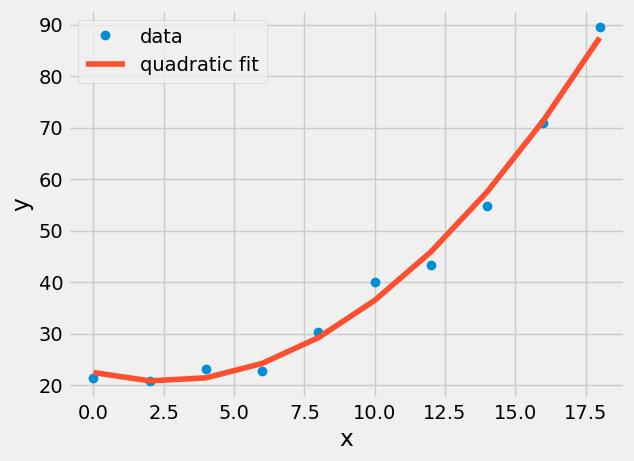
array([ 0.2763447 , -1.36268939, 22.46690909])

x_fcn=np.linspace(min(x),max(x));
plt.plot(x,y,'o',label='data')
plt.plot(x,Z@a,label='quadratic fit')
plt.xlabel('x')
plt.ylabel('y')
plt.legend();

Exercise

The quadratic curve plotted should be smooth, but matplotlib connected each (x,y)-location provided with straight lines. Plot the quadratic fit with 50 x-data points to make it smooth.

General Coefficient of Determination

The coefficient of determination is a measure of how much the standard deviation is due to random error when the data is fit to a function. You make the assumption that the data has some underlying correlation in the form of a function \(\mathbf{y}=f(\mathbf{x})\). So if you subtract the measured \(\mathbf{y}-f(\mathbf{x})\) the result should be random error associated with noise [4].

The general coefficient of determination is defined as \(r^2\),

\(r^{2}=\frac{S_{t}-S_{r}}{S_{t}}=1-\frac{S_{r}}{S_t}\)

where \(r\) is the correlation coefficient, \(S_t\) is the standard deviation of the measured \(\mathbf{y}\), and \(S_r\) is the standard deviation of the residuals, \(\mathbf{e} = \mathbf{y}-f(\mathbf{x}) = \mathbf{y}-\mathbf{Za}\).

St=np.std(y)
Sr=np.std(y-Z@a)

r2=1-Sr/St;
r=np.sqrt(r2);

print('the coefficient of determination for this fit is {}'.format(r2))
print('the correlation coefficient this fit is {}'.format(r))

the coefficient of determination for this fit is 0.91119056038536
the correlation coefficient this fit is 0.9545630206462851

Discussion

What is the highest possible coefficient of determination? If its maximized, is that a good thing?

Exercise

Compare the coefficient of determination for a straight line (you have to do a fit) to the quadratic fit (done above). Which one is a better fit?

Overfitting Warning

Coefficient of determination reduction does not always mean a better fit

You will always increase the coefficient of determination and decrease the total sum of squares error by adding more terms to your function. This is called overfitting your data. It is especially evident in polynomial fits, because they can behave unpredictably with higher order terms.

Nanonindentation data engineering model vs higher-order fit

Now, use experimental data from some atomic force microscope nanoindentation of \(MoS_2\) [2]. One of the nanoidentation experimental data files is in the data folder (../data/mos2_afm.csv).

The experiment pushes an AFM tip into the center of a hole covered with a single layer of \(MoS_2\), 0.6-nm thick. A diagram is shown below.

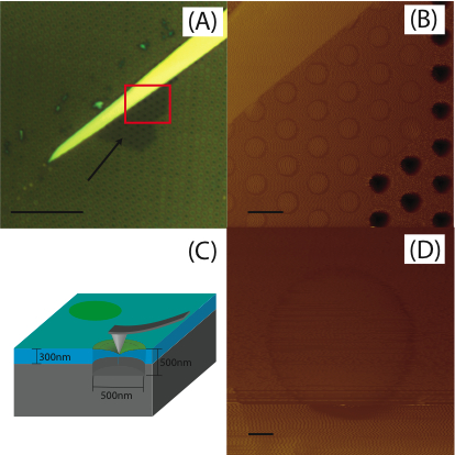
As the center of a thin sheet of \(MoS_2\) is pushed downwards the tension increases, resulting in higher measured force. An engineering equation for this increase in force is as such

\(F = A\delta + B \delta^3\)

where \(\delta\) is the deflection of the sheet (z in the data), \(A=\pi\sigma_0t\), \(B=1.09Et/r^2\), \(\sigma_0\) is the prestress in the sheet, \(E\) is the Young’s modulus, \(t=0.6~nm\) is the thickness, and \(r=260~nm\) is the radius of the sheet (they youre designed to be 250 nm, but there is some variation in microfabrication).

! head ../data/mos2_afm.csv

Z (nm),F (nN)
0,0
-0.011669,0.9
-0.0058346,0.45
0.3075,-1.35
0.29583,-0.45
0.5725,1.35
0.57833,0.9
0.5607,2.26
0.85666,1.8

Build a statistical model with Python’s Statsmodel

In the first Linear regression example in linear algebra, you built the \(\mathbf{Z}\) matrix and set up the least squares problem in the form

\(\mathbf{Z}^T\mathbf{ZA} = \mathbf{Z}^T\mathbf{y}\).

Now, try using the statsmodel.ols ordinary least squares statistical model solution. You use ols in two steps

1. build the model with the function and the measurements, \(\mathbf{Z}~and~\mathbf{y}\)

2. use the fit function to get statistical information about your best-fit model

import statsmodels.api as sm

mos2 = np.loadtxt('../data/mos2_afm.csv',delimiter=',',skiprows=1)
d = mos2[:,0] # deflection data
F = mos2[:,1] # force data
Z = d[:, np.newaxis]**[3, 1]
y = F

model = sm.OLS(y, Z)

---------------------------------------------------------------------------
ModuleNotFoundError                       Traceback (most recent call last)
Cell In[9], line 1
----> 1 import statsmodels.api as sm
      3 mos2 = np.loadtxt('../data/mos2_afm.csv',delimiter=',',skiprows=1)
      4 d = mos2[:,0] # deflection data

ModuleNotFoundError: No module named 'statsmodels'

Now, you have a variable, model, that contains the measured values of force and assumed function, \(F=A_0 \delta^3 + A_1 \delta^1\). Save the statistical output in the variable results. The statsmodel fit contains a lot of information. For now, look at two of the outputs

1. results.params: the coefficients \(A_0~and~A_1\)

2. results.summary: a statistical report on the best-fit model including

   • standard error of coefficients, std error

   • coefficient of determination R-squared

results = model.fit()
A = results.params
print('coeffictients are A0 = {}, A1 = {}'.format(*A))
print('Statsmodel summary of model')
plt.plot(d, F)
plt.plot(d,F,'.',label='afm data')
plt.plot(d,Z@results.params,label='best fit curve')
plt.title('Best fit curve and AFM data')
plt.xlabel('deflection (nm)')
plt.ylabel('Force (nN)')
plt.legend();
results.summary()

results?

print('Youngs modulus from fit = {:.0f} GPa'.format(A[0]/1.09/0.61*260**2))
print('Youngs modulus reported = 210 GPa')

Beyond polynomials

Linear Regression is only limited by the ability to separate the parameters from the function to achieve

\(\mathbf{y}=[\mathbf{Z}]\mathbf{a}\)

\(\mathbf{Z}\) can be any function of the independent variable(s).

Example: Let’s take some voltage-vs-time data that you know has two frequency components, \(\sin(t)\) and \(\sin(3t)\). You want to know what amplitudes are associated with each signal.

\(\mathbf{V}_{measured}=[\sin(t) \sin(3t)][amp_{1t},~amp_{3t}]^T\)

sin_data = np.loadtxt('../data/sin_data.csv')
t = sin_data[0,:];
V = sin_data[1,:];
plt.plot(t,V)
plt.xlabel('time (s)')
plt.ylabel('voltage (V)');

Z = np.block([[np.sin(t)],[np.sin(3*t)]]).T
model = sm.OLS(V, Z)
results = model.fit()
amps = results.params

plt.plot(t, V, 's')
plt.plot(t, Z@amps)
plt.title('Amplitudes of sin(t) and sin(3t) signals\n {:.3f} V and {:.3f} V'.format(*amps));

Fitting the Global Temperature Anomolies again

Now, you have the right tools to fit our Global temperature anomolies properly. Let’s create a function with three constants

\(f(t)= A\cdot t+B+ C\cdot H(t-1970)(t)\)

Where, \(A\) is the slope from time 1880-1970, B is the intercept (extrapolated temp anomoly at 0 A.D.), and C is the increase in slope after 1970, activated with a heaviside function, \(H(t-1970)=\) t>=1970. Our regression is still linear because each constant can be pulled out of our function to form \(\mathbf{Z}\).

\(\mathbf{Temp} = [t~~t^0~~(t-1970)\cdot H(t-1970)][A,~B,~C]^T\)

fname = '../data/land_global_temperature_anomaly-1880-2016.csv'

temp_data = pd.read_csv(fname,skiprows=4)

t = temp_data['Year'].values
T = temp_data['Value'].values

Z= np.block([[t],[t**0],[(t-1970)*(t>=1970)]]).T

print('This is every 10th row of Z')
print('---------------------------')
print(Z[::10])

fit = np.linalg.solve(Z.T@Z,Z.T@T)
#print(Z)

plt.plot(t,T,'o-',label='measured anomoly')
plt.plot(t,Z@fit,label='piece-wise best-fit')
plt.title('Piecewise fit to temperature anomoly')
plt.legend();

What You’ve Learned

• How to use the general least squares regression method for almost any function

• How to calculate the coefficient of determination and correlation coefficient for a general least squares regression, \(r^2~ and~ r\)

• Why you need to avoid overfitting

• How to construct general least squares regression using the dependent and independent data to form \(\mathbf{y}=\mathbf{Za}\).

• How to construct a piecewise linear regression

References

1. Numpy polyfit documentation

2. Cooper et. al 2014. Nonlinear Elastic Constants of \(MoS_2\). Phys. Rev. B 2013.

3. Figueroa et al. Stress Relaxation and Creep Recovery Tests Performed on Wheat Kernels Versus Doughs: Influence of Glutenins on Rheological and Quality Properties.

4. Chapra, Steven Applied Numerical Methods with Matlab for Engineers. ch 14. McGraw Hill.

5. Koerson, William. Overfitting vs. Underfitting: A Complete Example