Content modified under Creative Commons Attribution license CC-BY 4.0, code under BSD 3-Clause License © 2020 R.C. Cooper, L.A. Barba, N.C. Clementi
04 - Statistics and Monte-Carlo Models#
Monte Carlo models use random numbers to either understand statistics or generate a solution [1]. The main element in a Monte Carlo model is the use of random numbers. Monte Carlo methods are very useful if you can easily execute a function lots of time or even in parallel.
We can generate random numbers in many ways, but most programming languages have ‘pseudo’-random number generators.
In Python, we use the NumPy random library as such
import numpy as np
from numpy.random import default_rng
rng = default_rng()

x = rng.random(20)
x
array([0.418836  , 0.75823529, 0.96328367, 0.57404585, 0.89434351,
       0.43697919, 0.31922792, 0.27086855, 0.5921934 , 0.57226881,
       0.2104138 , 0.35796936, 0.40788707, 0.93015879, 0.22947006,
       0.55762363, 0.93467438, 0.20307222, 0.39155015, 0.67284354])
NumPy’s random number generator (rng) creates random numbers that can
be uniformly
distributed,
normally
distributed, and
much
more.
The call to rng.random(20) created 20 uniformly random numbers between
0 and 1 saved as the variable x. Next, you can plot the histogram of
x.
import matplotlib.pyplot as plt
plt.style.use('fivethirtyeight')
plt.hist(x, bins = 5,
            color = 'b',
            histtype = 'bar',
            edgecolor = 'w')
(array([5., 5., 4., 2., 4.]),
 array([0.20307222, 0.35511451, 0.5071568 , 0.65919909, 0.81124138,
        0.96328367]),
 <BarContainer object of 5 artists>)
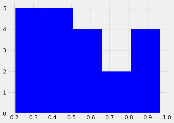
The pyplot function hist displays a histogram of these randomly generated numbers.
Exercise and Discussion#
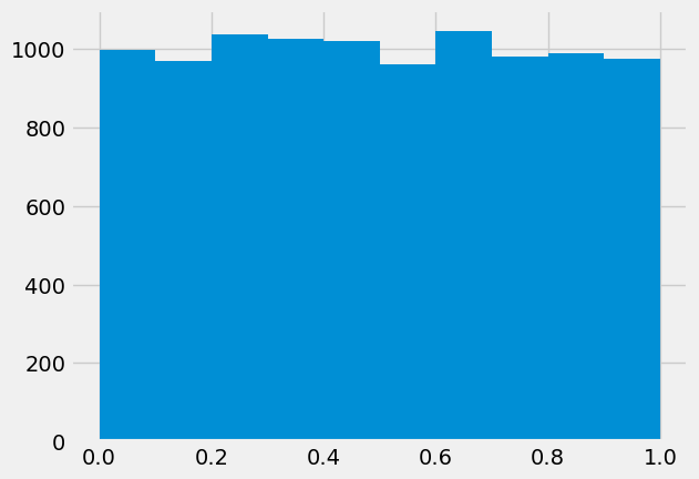
Try generating more random numbers and plotting histograms of the results i.e. increase 10 to larger values.
What should the histogram of x look like if Python is generating truly random numbers?
rng = default_rng()
x = rng.random(10000)
plt.hist(x);
Examples of Monte Carlo models:#
Monte Carlo models have a wide array of applications. We are going to use Monte Carlo models in later modules to explore how uncertainty in measurements can be incorporated into computational models. The three main applications for Monte Carlo models are used in three main classes: optimization, numerical integration, and generating population distributions [1].
Here is a brief list of Monte Carlo model use cases in real-world applications:
disordered materials (physics)
We will explore Monte Carlo modeling through the use of three examples:
Calculate the value of \(\pi\)
Simulate Brownian motion of particles in fluids
Propagate uncertainty in manufacturing into uncertainty in failure load
Example 1: Calculate \(\pi\) with random numbers.#
Assuming we can actually generate random numbers (a topic of philosophical and heated debates) we can populate a unit square with random points and determine the ratio of points inside and outside of a circle.
The ratio of the area of the circle to the square is:
\(\frac{\pi r^{2}}{4r^{2}}=\frac{\pi}{4}\)
So if we know the fraction of random points that are within the unit circle, then we can calculate \(\pi\)
(number of points in circle)/(total number of points)=\(\pi/4\)
def montecarlopi(N):
    '''Create random x-y-coordinates to and use ratio of circle-to-square to
    calculate the value of pi
    i.e. Acircle/Asquare = pi/4
    Arguments
    ---------
    N: number of random points to produce between x=0-1 and y=0-1

    Returns
    -------
    our_pi: the best prediction of pi using N points
    '''


    x = rng.random(N);
    y = rng.random(N);
    R=np.sqrt(x**2+y**2); # compute radius
    num_in_circle=sum(R<1);
    total_num_pts =len(R);
    our_pi = 4*num_in_circle/total_num_pts;
    return our_pi
test_pi=np.zeros(10)
for i in range(0,10):
    test_pi[i]=montecarlopi(1000);

print('mean value for pi = %f'%np.mean(test_pi))
print('standard deviation is %f'%np.std(test_pi))
print('actual pi is %f'%np.pi)
mean value for pi = 3.144400
standard deviation is 0.042987
actual pi is 3.141593
Exercises#
Why is there a standard deviation for the value of \(\pi\) calculated with a Monte Carlo method? Does it depend upon how many times you run the function i.e. the size of
test_pi? or the number of random pointsN? Alter the script above to discover correlationsHow well does your function
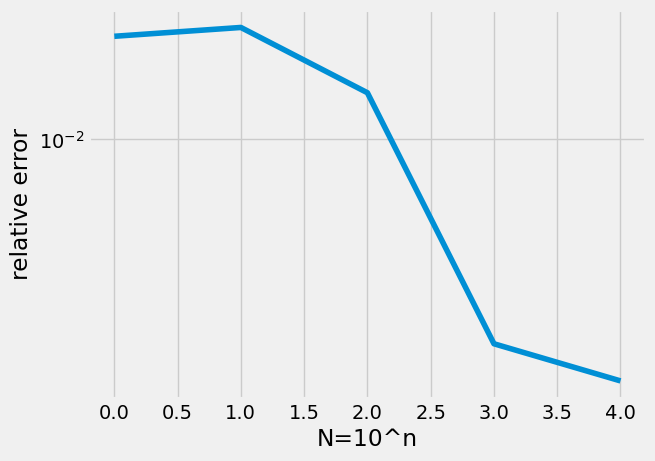
montecarlopiconverge to the true value of \(\pi\) (you can usenp.pias a true value)? Plot the convergence as we did in 03-Numerical_error
test_pi=np.zeros(100)
for i in range(0,100):
    test_pi[i]=montecarlopi(1000);

print('mean value for pi = %f'%np.mean(test_pi))
print('standard deviation is %f'%np.std(test_pi))
print('actual pi is %f'%np.pi)
mean value for pi = 3.145000
standard deviation is 0.047814
actual pi is 3.141593
Compare the above 100 test_pi cases each 1000 points.
to the below 10 test_pi cases each 10,000 points.
Above, the std is the same as before \(\approx 0.05\)
Below, the std is decreased to \(\approx 0.01\)
test_pi=np.zeros(10)
for i in range(0,10):
    test_pi[i]=montecarlopi(10000);

print('mean value for pi = %f'%np.mean(test_pi))
print('standard deviation is %f'%np.std(test_pi))
print('actual pi is %f'%np.pi)
mean value for pi = 3.137200
standard deviation is 0.014397
actual pi is 3.141593
N=np.arange(0,5)
error = np.zeros(len(N))

for n in N:
    mypi = np.zeros(10)
    for i in range(0,10):
        mypi[i]=montecarlopi(10**n)
    mupi = np.mean(mypi)
    error[n] = np.abs(np.pi-mupi)/np.pi
plt.semilogy(N,error)
plt.xlabel('N=10^n')
plt.ylabel('relative error');
Example 2: Simulate Brownian motion of particles in a fluid#
Brownian motion was first documented by Robert Brown, a Scottish botanist in 1827. It is a description of how large particles move and vibrate in fluids that have no buld motion. The atoms from the fluid bounce off the suspended particles to jiggle them randomly left and right. Take a look at Up and Atom’s video for more information in the physics and history of the phenomenon.
from IPython.display import YouTubeVideo
YouTubeVideo('5jBVYvHeG2c')
In this example, your goal is to predict the location of 50 particles if they take 100 random steps from -0.5 to 0.5 \(\mu m\) in the x- and y-directions.
Exercise (Discussion)#
If the steps are uniformly random and can be positive or negative, where do you expect the particle to be after 100 steps? Will it be back to where it started? or will it migrate to somewhere new?
Generate your Brownian motion#
Here, we are simplifying the physics of the Brownian motion (ignoring the details in the transfer of momentum from small to large particles) and just assuming each step in the x- and y-directions are -0.5 to 0.5 \(\mu m\). Here is the Monte Carlo process:
generate 2 sets of 100 random numbers between -0.5 to 0.5 for \(Delta x\) and \(\Delta y\).
create an array with 100 locations, the first is at the origin (0, 0)
take a cumulative sum of the \(\Delta x\) and \(\Delta y\) steps to find the location at each step
plot the results
Here, you create the 100 random numbers and shift them by 0.5.
rng = default_rng()
N_steps = 100
dx = rng.random(N_steps) - 0.5
dy = rng.random(N_steps) - 0.5
Next, create the positions at each step.
r = np.zeros((N_steps, 2))
Now, use
np.cumsum
to find the final position after each step is taken.
r[:, 0] = np.cumsum(dx) # final rx position
r[:, 1] = np.cumsum(dy) # final ry position
Finally, you can plot the path the particle took as it moved along its 100 steps and its final location.
plt.plot(r[:, 0 ], r[:, 1])
plt.plot(r[-1, 0], r[-1, 1], 'o', markersize = 10)
plt.xlabel('x-position (um)')
plt.ylabel('y-position (um)')
Text(0, 0.5, 'y-position (um)')
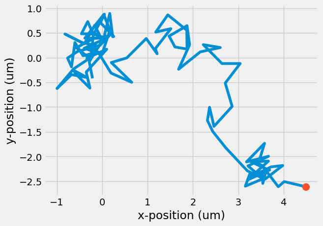
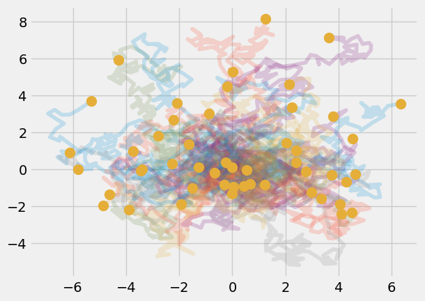
A curious result, even though we prescribed random motion, the final location did not end up back at the origin, where it started. What if you looked at 50 particles? How many would end up back at the origin? Use a for-loop to calculate the position of 50 particles taking 100 steps each.
num_particles = 50
r_final = np.zeros((num_particles, 2))
for i in range(0, num_particles):
    dx = rng.random(N_steps) - 0.5
    dy = rng.random(N_steps) - 0.5

    r = np.zeros((N_steps, 2))

    r[:, 0] = np.cumsum(dx)
    r[:, 1] = np.cumsum(dy)
    r_final[i, :] = r[-1, :]

    plt.plot(r[:, 0 ], r[:, 1], alpha = 0.2)
plt.plot(r_final[:, 0], r_final[:, 1], 'o', markersize = 10)
[<matplotlib.lines.Line2D at 0x7f41d04fb090>]
Exercise#
Calculate the average location of the particles. What is the standard deviation?
Exercise#
Compare the scaled histogram to the original histogram. What is similar? What is different?
Make a scaling equation to get uniformly random numbers between 10 and 20.
The scaling keeps the bin heights constant, but it changes the width and location of the bins in the histogram. Scaling to 10-20 shows a more extreme example.
Example 3: Determine uncertainty in failure load based on geometry uncertainty#
In this example, we know that a steel bar will break under 940 MPa tensile stress. The bar is 1 mm by 2 mm with a tolerance of 10 %. What is the range of tensile loads that can be safely applied to the beam?
\(\sigma_{UTS}=\frac{F_{fail}}{wh}\)
\(F_{fail}=\sigma_{UTS}wh\)
N = 10000
r = rng.random(N)
wmean = 1 # in mm
wmin = wmean-wmean*0.1
wmax = wmean+wmean*0.1
hmean = 2 # in mm
hmin = hmean-hmean*0.1
hmax = hmean+hmean*0.1
wrand=wmin+(wmax-wmin)*r
hrand=hmin+(hmax-hmin)*r
uts=940 # in N/mm^2=MPa
Ffail=uts*wrand*hrand*1e-3 # force in kN
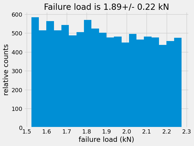
plt.hist(Ffail,bins=20,)
plt.xlabel('failure load (kN)')
plt.ylabel('relative counts')
plt.title('Failure load is {:.2f}+/- {:.2f} kN'.format(np.mean(Ffail),np.std(Ffail)))
Text(0.5, 1.0, 'Failure load is 1.89+/- 0.22 kN')
Normally, the tolerance is not a maximum/minimum specification, but instead a normal distribution that describes the standard deviation, or the 68% confidence interval.
So instead, you should generate normally distributed dimensions.
N=10000
wmean=1 # in mm
wstd=wmean*0.1 # standard deviation in mm
hmean=2 # in mm
hstd=hmean*0.1 # standard deviation in mm


wrand=rng.normal(loc = wmean, scale = wstd, size = N)
hrand=np.random.normal(loc = hmean, scale = hstd, size = N)
uts=940 # in N/mm^2=MPa

Ffail=uts*wrand*hrand*1e-3 # force in kN
plt.hist(Ffail,bins=20)
#plt.xlabel('failure load (kN)')
#plt.ylabel('relative counts')
plt.title('Failure load is {:.2f}+/- {:.2f} kN'.format(np.mean(Ffail),np.std(Ffail)))
Text(0.5, 1.0, 'Failure load is 1.88+/- 0.26 kN')
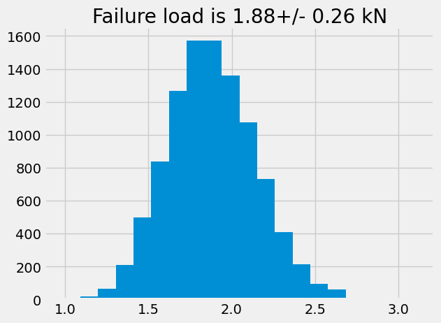
In this propagation of uncertainty, the final value of failure load seems to be independent of wheher the distribution is uniformly random or normally distributed. In both cases, the failure load is \(\approx 1.9 \pm 0.25\) kN.
The difference is much more apparent if you look at the number of occurrences that failure will occur whether the dimensions are uniformly random or normally distributed.
For the uniformly random case, there are approximately 500 parts out of 10,000 that will fail at 1.9 kN.
For the normally distributed case, there are approximately 1500 parts out of 10,000 that will fail at 1.9 kN.
What you’ve learned:#
How to generate “random” numbers in Python\(^+\)
The definition of a Monte Carlo model
How to calculate \(\pi\) with Monte Carlo
How to model Brownian motion with Monte Carlo
How to propagate uncertainty in a model with Monte Carlo
\(^+\) Remember, the computer only generates pseudo-random numbers. For further information and truly random numbers check www.random.org
References#
Meurer A, et al. (2017) SymPy: symbolic computing in Python. PeerJ Computer Science 3:e103 https://doi.org/10.7717/peerj-cs.103
Whittaker, E. T. and Robinson, G. “Normal Frequency Distribution.” Ch. 8 in The Calculus of Observations: A Treatise on Numerical Mathematics, 4th ed. New York: Dover, p. 179, 1967.