02 - Working with Python

Content modified under Creative Commons Attribution license CC-BY 4.0, code under BSD 3-Clause License © 2020 R.C. Cooper

02 - Working with Python#

Good coding habits#

naming folders and files#

Stanford file naming best practices #

Include information to distinguish file name e.g. project name, objective of function, name/initials, type of data, conditions, version of file,
if using dates, use YYYYMMDD, so the computer organizes by year, then month, then day
avoid special characters e.g. !, #, $, …
avoid using spaces if not necessary, some programs consider a space as a break in code use dashes - or underscores _ or CamelCase

Commenting your code#

Its important to comment your code

what are variable’s units,
what the is the function supposed to do,
etc.

def code(i):
    '''Example of bad variable names and bad function name'''
    m=1
    for j in range(1,i+1):
        m*=j;
    return m

code(10)

Choose variable names that describe the variable#

You might not have recognized that code(i) is meant to calculate the factorial of a number,

$N!= N*(N-1)*(N-2)*(N-3)*...3*2*1$.

For example,

4! = 24
5! = 120
10! = 3,628,800

In the next block, code is rewritten and the output is unchanged, but another user can read the code and help debug if there is an issue.

A function is a compact collection of code that executes some action on its arguments.

Once defined, you can call a function as many times as you want. When you call a function, you execute all the code inside the function. The result of the execution depends on the definition of the function and on the values that are passed into it as arguments. Functions might or might not return values in their last operation.

The syntax for defining custom Python functions is:

def function_name(arg_1, arg_2, ...):
    '''
    docstring: description of the function
    '''
    <body of the function>

The docstring of a function is a message from the programmer documenting what he or she built. Docstrings should be descriptive and concise. They are important because they explain (or remind) the intended use of the function to the users. You can later access the docstring of a function using the function help() and passing the name of the function. If you are in a notebook, you can also prepend a question mark '?' before the name of the function and run the cell to display the information of a function.

Try it!

def factorial_function(input_value):
    '''Good variable names and better help documentation
     
    factorial_function(input_number): calculates the factorial of the input_number
    where the factorial is defined as N*(N-1)*(N-2)*...*3*2*1
    
    Arguments
    ---------
    input_value: an integer >= 0
    
    Returns
    -------
    factorial_output: the factorial of input_value'''
    
    factorial_output=1 # define 0! = 1
    for factor in range(1,input_value+1):
        factorial_output*=factor; # mutliply factorial_output by 1*2*3*...*N (factor)
    return factorial_output
         

factorial_function(4)

Defining the function with descriptive variable names and inputs helps to make the function much more useable.

Consider the structure of a Python function:

def factorial_function(input_value):

This first line declares that you are def-ining a function that is named factorial_function. The inputs to the line are given inside the parantheses, (input_value). You can define as many inputs as we want and even assign default values.

    '''Good variable names and better help documentation
     
    factorial_function(input_number): calculates the factorial of the input_number
    where the factorial is defined as N*(N-1)*(N-2)*...*3*2*1'''

The next 4 lines define a help documentation that can be accessed with in a couple ways:

?factorial_function
factorial_function?
help(factorial_function)

factorial_function?

    factorial_output=1 # define 0! = 1

This line sets the variable factorial_output to 1. In the next 2 lines update this value based upon the mathematical formula we want to use. In this case, its $1*1*2*3*...*(N-1)*N$

    for factor in range(1,input_value+1):
        factorial_output*=factor; # mutliply m by 1*2*3*...*N (factor)

These two lines perform the computation that you set out to do. The for-loop is going to start at 1 and end at our input value. For each step in the for-loop, we will mulitply the factorial_output by the factor. So when you calculate $4!$, the loop updates factorial_output 4 times:

i=1: factorial_output = $1*1=1$
i=2: factorial_output = $1*1*2=2$
i=3: factorial_output = $1*1*2*3=6$
i=4: factorial_output = $1*1*2*3*4=24$

    return factorial_output

This final line in our function returns the calculated value, factorial_output. You can also return as many values as necessary on this line,

for example, if you had variables: value_1, value_2, and value_3 you could return all three as such,

    return value_1,value_2,value_3

Play with NumPy Arrays#

In engineering applications, most computing situations benefit from using arrays: they are sequences of data all of the same type. They behave a lot like lists, except for the constraint in the type of their elements. There is a huge efficiency advantage when you know that all elements of a sequence are of the same type—so equivalent methods for arrays execute a lot faster than those for lists.

The Python language is expanded for special applications, like scientific computing, with libraries. The most important library in science and engineering is NumPy, providing the n-dimensional array data structure (a.k.a, ndarray) and a wealth of functions, operations and algorithms for efficient linear-algebra computations.

In this lesson, you’ll start playing with NumPy arrays and discover their power. You’ll also meet another widely loved library: Matplotlib, for creating two-dimensional plots of data.

Importing libraries#

First, a word on importing libraries to expand your running Python session. Because libraries are large collections of code and are for special purposes, they are not loaded automatically when you launch Python (or IPython, or Jupyter). You have to import a library using the import command. For example, to import NumPy, with all its linear-algebra goodness, you enter:

import numpy as np

Once you execute that command in a code cell, you can call any NumPy function using the dot notation, prepending the library name. For example, some commonly used functions are:

Follow the links to explore the documentation for these very useful NumPy functions!

import numpy as np

Creating arrays#

To create a NumPy array from an existing list of (homogeneous) numbers, you call np.array(), like this:

np.array([3, 5, 8, 17])

array([ 3,  5,  8, 17])

NumPy offers many ways to create arrays in addition to this. Some of them above.

Play with np.ones() and np.zeros(): they create arrays full of ones and zeros, respectively. You pass as an argument the number of array elements we want.

np.ones(5)

array([1., 1., 1., 1., 1.])

np.zeros(3)

array([0., 0., 0.])

Another useful one: np.arange() gives an array of evenly spaced values in a defined interval.

Syntax:

np.arange(start, stop, step)

where start by default is zero, stop is not inclusive, and the default for step is one. Play with it!

np.arange(4)

array([0, 1, 2, 3])

np.arange(2, 6)

array([2, 3, 4, 5])

np.arange(2, 6, 2)

array([2, 4])

np.arange(2, 6, 0.5)

array([2. , 2.5, 3. , 3.5, 4. , 4.5, 5. , 5.5])

np.linspace() is similar to np.arange(), but uses number of samples instead of a step size. It returns an array with evenly spaced numbers over the specified interval.

Syntax:

np.linspace(start, stop, num)

stop is included by default (it can be removed, read the docs), and num by default is 50.

np.linspace(2.0, 3.0)

array([2.        , 2.02040816, 2.04081633, 2.06122449, 2.08163265,
       2.10204082, 2.12244898, 2.14285714, 2.16326531, 2.18367347,
       2.20408163, 2.2244898 , 2.24489796, 2.26530612, 2.28571429,
       2.30612245, 2.32653061, 2.34693878, 2.36734694, 2.3877551 ,
       2.40816327, 2.42857143, 2.44897959, 2.46938776, 2.48979592,
       2.51020408, 2.53061224, 2.55102041, 2.57142857, 2.59183673,
       2.6122449 , 2.63265306, 2.65306122, 2.67346939, 2.69387755,
       2.71428571, 2.73469388, 2.75510204, 2.7755102 , 2.79591837,
       2.81632653, 2.83673469, 2.85714286, 2.87755102, 2.89795918,
       2.91836735, 2.93877551, 2.95918367, 2.97959184, 3.        ])

len(np.linspace(2.0, 3.0))

np.linspace(2.0, 3.0, 6)

array([2. , 2.2, 2.4, 2.6, 2.8, 3. ])

np.linspace(-1, 1, 9)

array([-1.  , -0.75, -0.5 , -0.25,  0.  ,  0.25,  0.5 ,  0.75,  1.  ])

Array operations#

Let’s assign some arrays to variable names and perform some operations with them.

x_array = np.linspace(-1, 1, 9)

Now that you’ve saved it with a variable name, you can do some computations with the array. For example, take the square of every element of the array, in one go:

y_array = x_array**2
print(y_array)

[1.     0.5625 0.25   0.0625 0.     0.0625 0.25   0.5625 1.    ]

You can also take the square root of a positive array, using the np.sqrt() function:

z_array = np.sqrt(y_array)
print(z_array)

[1.   0.75 0.5  0.25 0.   0.25 0.5  0.75 1.  ]

Now that you have different arrays x_array, y_array and z_array, you can do more computations, like add or multiply them. For example:

add_array = x_array + y_array 
print(add_array)

[ 0.     -0.1875 -0.25   -0.1875  0.      0.3125  0.75    1.3125  2.    ]

Array addition is defined element-wise, like when adding two vectors (or matrices). Array multiplication is also element-wise:

mult_array = x_array * z_array
print(mult_array)

[-1.     -0.5625 -0.25   -0.0625  0.      0.0625  0.25    0.5625  1.    ]

You can also divide arrays, but you have to be careful not to divide by zero. This operation will result in a nan which stands for Not a Number. Python will still perform the division, but will tell us about the problem.

Let’s see how this might look:

x_array / y_array

/tmp/ipykernel_1909/2664324349.py:1: RuntimeWarning: invalid value encountered in divide
  x_array / y_array

array([-1.        , -1.33333333, -2.        , -4.        ,         nan,
        4.        ,  2.        ,  1.33333333,  1.        ])

Multidimensional arrays#

2D arrays#

NumPy can create arrays of N dimensions. For example, a 2D array is like a matrix, and is created from a nested list as follows:

array_2d = np.array([[1, 2], [3, 4]])
print(array_2d)

[[1 2]
 [3 4]]

2D arrays can be added, subtracted, and multiplied:

X = np.array([[1, 2], [3, 4]])
Y = np.array([[1, -1], [0, 1]])

The addition of these two matrices works exactly as you would expect:

X + Y

array([[2, 1],
       [3, 5]])

What if you try to multiply arrays using the '*'operator?

X * Y

array([[ 1, -2],
       [ 0,  4]])

The multiplication using the '*' operator is element-wise. If you want to do matrix multiplication use the '@' operator:

X @ Y

array([[1, 1],
       [3, 1]])

Or equivalently use np.dot():

np.dot(X, Y)

array([[1, 1],
       [3, 1]])

3D arrays#

Let’s create a 3D array by reshaping a 1D array. You can use np.reshape(), where you pass the array we want to reshape and the shape we want to give it, i.e., the number of elements in each dimension.

Syntax

np.reshape(array, newshape)

For example:

a = np.arange(24)

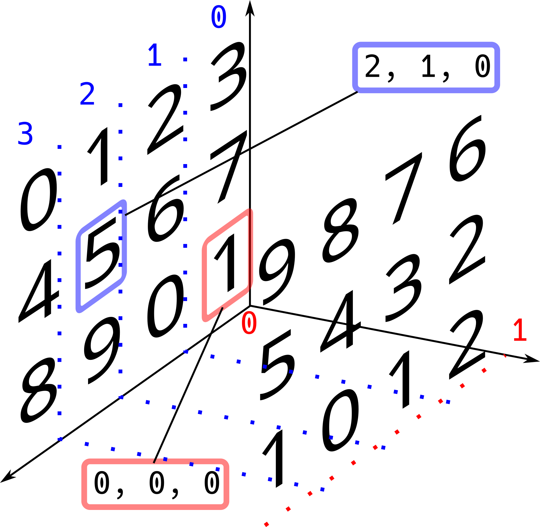
a_3D = np.reshape(a, (2, 3, 4))
print(a_3D)

[[[ 0  1  2  3]
  [ 4  5  6  7]
  [ 8  9 10 11]]

 [[12 13 14 15]
  [16 17 18 19]
  [20 21 22 23]]]

You can check for the shape of a NumPy array using the function np.shape():

np.shape(a_3D)

(2, 3, 4)

Visualizing the dimensions of the a_3D array can be tricky, so here is a diagram that will help you to understand how the dimensions are assigned: each dimension is shown as a coordinate axis. For a 3D array, on the “x axis”, you have the sub-arrays that themselves are two-dimensional (matrices). Two of these 2D sub-arrays, in this case; each one has 3 rows and 4 columns. Study this sketch carefully, while comparing with how the array a_3D is printed out above.

A 3D array with two 3x4 matrices extended along a thirddimension

When you have multidimensional arrays, you can access slices of their elements by slicing on each dimension. This is one of the advantages of using arrays: you cannot do this with lists.

Let’s access some elements of our 2D array called X.

array([[1, 2],
       [3, 4]])

# Grab the element in the 1st row and 1st column 
X[0, 0]

# Grab the element in the 1st row and 2nd column 
X[0, 1]

Exercises:#

From the X array:

Grab the 2nd element in the 1st column.
Grab the 2nd element in the 2nd column.

Play with slicing on this array:

# Grab the 1st column
X[:, 0]

array([1, 3])

When you don’t specify the start and/or end point in the slicing, the symbol ':' means “all”. In the example above, you are telling NumPy that we want all the elements from the 0-th index in the second dimension (the first column).

# Grab the 1st row
X[0, :]

array([1, 2])

Exercises:#

From the X array:

Grab the 2nd column.
Grab the 2nd row.

Let’s practice with a 3D array.

a_3D

array([[[ 0,  1,  2,  3],
        [ 4,  5,  6,  7],
        [ 8,  9, 10, 11]],

       [[12, 13, 14, 15],
        [16, 17, 18, 19],
        [20, 21, 22, 23]]])

If you want to grab the first column of both matrices in our a_3D array, do:

a_3D[:, :, 0]

array([[ 0,  4,  8],
       [12, 16, 20]])

The line above is telling NumPy that you want:

first ':' : from the first dimension, grab all the elements (2 matrices).
second ':': from the second dimension, grab all the elements (all the rows).
'0' : from the third dimension, grab the first element (first column).

If you want the first 2 elements of the first column of both matrices:

a_3D[:, 0:2, 0]

array([[ 0,  4],
       [12, 16]])

Below, from the first matrix in our a_3D array, you will grab the two middle elements (5,6):

a_3D[0, 1, 1:3]

array([5, 6])

Exercises:#

From the array named a_3D:

Grab the two middle elements (17, 18) from the second matrix.
Grab the last row from both matrices.
Grab the elements of the 1st matrix that exclude the first row and the first column.
Grab the elements of the 2nd matrix that exclude the last row and the last column.

NumPy == Fast and Clean!#

When you are working with numbers, arrays are a better option because the NumPy library has built-in functions that are optimized, and therefore faster than vanilla Python. Especially if we have big arrays. Besides, using NumPy arrays and exploiting their properties makes our code more readable.

For example, if you wanted to add element-wise the elements of 2 lists, you need to do it with a for statement. If you want to add two NumPy arrays, you just use the addtion '+' symbol!

Below, you will add two lists and two arrays (with random elements) and you’ll compare the time it takes to compute each addition.

Element-wise sum of a Python list#

Using the Python library random, you will generate two lists with 100 pseudo-random elements in the range [0,100), with no numbers repeated.

#import random library
import random

lst_1 = random.sample(range(100), 100)
lst_2 = random.sample(range(100), 100)

#print first 10 elements
print(lst_1[0:10])
print(lst_2[0:10])

[28, 69, 74, 93, 62, 7, 36, 92, 76, 43]
[4, 61, 24, 47, 57, 59, 8, 86, 22, 56]

We need to write a for statement, appending the result of the element-wise sum into a new list you call result_lst.

For timing, you can use the IPython “magic” %%time. Writing at the beginning of the code cell the command %%time will give us the time it takes to execute all the code in that cell.

%%time
res_lst = []
for i in range(100):
    res_lst.append(lst_1[i] + lst_2[i])

CPU times: user 11 µs, sys: 8 µs, total: 19 µs
Wall time: 21.7 µs

print(res_lst[0:10])

[32, 130, 98, 140, 119, 66, 44, 178, 98, 99]

Element-wise sum of NumPy arrays#

In this case, you generate arrays with random integers using the NumPy function np.random.randint(). The arrays you generate with this function are not going to be like the lists: in this case you’ll have 100 elements in the range [0, 100) but they can repeat. Our goal is to compare the time it takes to compute addition of a list or an array of numbers, so all that matters is that the arrays and the lists are of the same length and type (integers).

arr_1 = np.random.randint(0, 100, size=100)
arr_2 = np.random.randint(0, 100, size=100)

#print first 10 elements
print(arr_1[0:10])
print(arr_2[0:10])

[33 50 53 89 13 74 41 74 95 42]
[31 32 59 10 98 16  9 67  1  6]

Now, you can use the %%time cell magic, again, to see how long it takes NumPy to compute the element-wise sum.

%%time
arr_res = arr_1 + arr_2

CPU times: user 6 µs, sys: 5 µs, total: 11 µs
Wall time: 12.9 µs

Notice that in the case of arrays, the code not only is more readable (just one line of code), but it is also faster than with lists. This time advantage will be larger with bigger arrays/lists.

(Your timing results may vary to the ones you show in this notebook, because you will be computing in a different machine.)

Exercise#

Try the comparison between lists and arrays, using bigger arrays; for example, of size 10,000.
Repeat the analysis, but now computing the operation that raises each element of an array/list to the power two. Use arrays of 10,000 elements.

Time to Plot#

You will love the Python library Matplotlib! You’ll learn here about its module pyplot, which makes line plots.

We need some data to plot. Let’s define a NumPy array, compute derived data using its square, cube and square root (element-wise), and plot these values with the original array in the x-axis.

xarray = np.linspace(0, 2, 41)
print(xarray)

[0.   0.05 0.1  0.15 0.2  0.25 0.3  0.35 0.4  0.45 0.5  0.55 0.6  0.65
 0.7  0.75 0.8  0.85 0.9  0.95 1.   1.05 1.1  1.15 1.2  1.25 1.3  1.35
 1.4  1.45 1.5  1.55 1.6  1.65 1.7  1.75 1.8  1.85 1.9  1.95 2.  ]

pow2 = xarray**2
pow3 = xarray**3
pow_half = np.sqrt(xarray)

Introduction to plotting#

To plot the resulting arrays as a function of the orginal one (xarray) in the x-axis, you need to import the module pyplot from Matplotlib.

import matplotlib.pyplot as plt

Set up default plotting parameters#

The default Matplotlib fonts and linewidths are a little small. Pixels are free, so the next two lines increase the fontsize and linewidth

plt.rcParams.update({'font.size': 22})
plt.rcParams['lines.linewidth'] = 3

The line %matplotlib inline is an instruction to get the output of plotting commands displayed “inline” inside the notebook. Other options for how to deal with plot output are available, but not of interest to you right now.

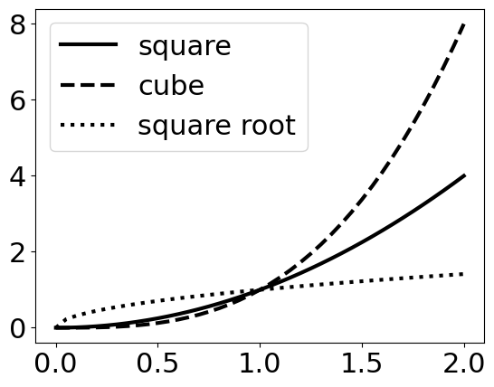
We’ll use the pyplot plt.plot() function, specifying the line color ('k' for black) and line style ('-', '--' and ':' for continuous, dashed and dotted line), and giving each line a label. Note that the values for color, linestyle and label are given in quotes.

#Plot x^2
plt.plot(xarray, pow2, color='k', linestyle='-', label='square')
#Plot x^3
plt.plot(xarray, pow3, color='k', linestyle='--', label='cube')
#Plot sqrt(x)
plt.plot(xarray, pow_half, color='k', linestyle=':', label='square root')
#Plot the legends in the best location
plt.legend(loc='best')

<matplotlib.legend.Legend at 0x7f696feba910>

../_images/81759b3a77c1d267dc07c97e4f544a3734b2f6456a1c80b25ca38178a22ada9a.png

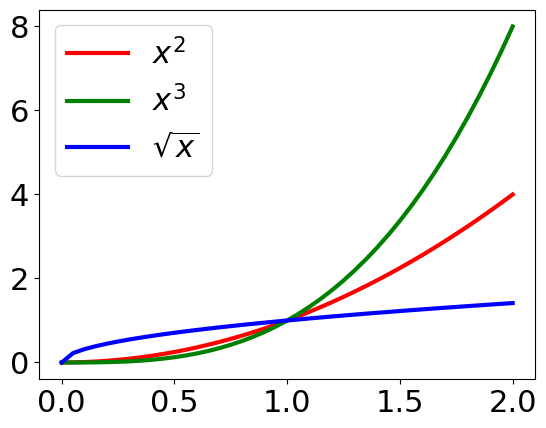
To illustrate other features, you will plot the same data, but varying the colors instead of the line style. We’ll also use LaTeX syntax to write formulas in the labels. If you want to know more about LaTeX syntax, there is a quick guide to LaTeX available online.

Adding a semicolon (';') to the last line in the plotting code block prevents that ugly output, like <matplotlib.legend.Legend at 0x7f8c83cc7898>. Try it.

#Plot x^2
plt.plot(xarray, pow2, color='red', linestyle='-', label='$x^2$')
#Plot x^3
plt.plot(xarray, pow3, color='green', linestyle='-', label='$x^3$')
#Plot sqrt(x)
plt.plot(xarray, pow_half, color='blue', linestyle='-', label='$\sqrt{x}$')
#Plot the legends in the best location
plt.legend(loc='best'); 

../_images/e022f3bdc65d63ee6d142db4ca44c03cb256a469e295d98baaa2419ac11f787a.png

That’s very nice! By now, you are probably imagining all the great stuff you can do with Jupyter notebooks, Python and its scientific libraries NumPy and Matplotlib. We just saw an introduction to plotting but you will keep learning about the power of Matplotlib in the next lesson.

If you are curious, you can explore all the beautiful plots you can make by browsing the Matplotlib gallery.

Exercise:#

Pick two different operations to apply to the xarray and plot them the resulting data in the same plot.

What you’ve learned#

Good coding habits and file naming
How to define a function and return outputs
How to import libraries
Multidimensional arrays using NumPy
Accessing values and slicing in NumPy arrays
%%time magic to time cell execution.
Performance comparison: lists vs NumPy arrays
Basic plotting with pyplot.

References#

Best practices for file naming. Stanford Libraries
Effective Computation in Physics: Field Guide to Research with Python (2015). Anthony Scopatz & Kathryn D. Huff. O’Reilly Media, Inc.
Numerical Python: A Practical Techniques Approach for Industry. (2015). Robert Johansson. Appress.
“The world of Jupyter”—a tutorial. Lorena A. Barba - 2016

02 - Working with Python

Contents

02 - Working with Python#

Good coding habits#

naming folders and files#

Stanford file naming best practices#

Commenting your code#

Choose variable names that describe the variable#

Play with NumPy Arrays#

Importing libraries#

Creating arrays#

Array operations#

Multidimensional arrays#

2D arrays#

3D arrays#

Exercises:#

Exercises:#

Exercises:#

NumPy == Fast and Clean!#

Element-wise sum of a Python list#

Element-wise sum of NumPy arrays#

Exercise#

Time to Plot#

Introduction to plotting#

Set up default plotting parameters#

Exercise:#

What you’ve learned#

References#

Stanford file naming best practices #