Project #02 - NYSE random walk predictor

Project #02 - NYSE random walk predictor#

In the Stats and Monte Carlo module, you created a Brownian motion model to predict the motion of particles in a fluid. The Monte Carlo model took steps in the x- and y-directions with random magnitudes.

This random walk can be used to predict stock prices. Let’s take a look at some data from the New York Stock Exchange NYSE from 2010 through 2017.

Important Note: I am not a financial advisor and these models are purely for academic exercises. If you decide to use anything in these notebooks to make financial decisions, it is at your own risk. I am not an economist/financial advisor/etc., I am just a Professor who likes to learn and exeriment.

Here, I will show an example workflow to analyze and predict the Google stock price [GOOGL] from 2010 - 2014. Then, you can choose your own stock price to evaluate and create a predictive model.

Explore data and select data of interest
Find statistical description of data: mean and standard deviation
Create random variables
Generate random walk for [GOOGL] stock opening price

1. Explore data#

Here, I load the data into a Pandas dataframe to see what headings and values are available. I see two columns that I want to analyze

‘date’
‘open’

data = pd.read_csv('../data/nyse-data.csv')
data['date'] = pd.to_datetime(data['date'])
data

---------------------------------------------------------------------------
ValueError                                Traceback (most recent call last)
Cell In[2], line 2
      1 data = pd.read_csv('../data/nyse-data.csv')
----> 2 data['date'] = pd.to_datetime(data['date'])
      3 data

File /opt/hostedtoolcache/Python/3.9.19/x64/lib/python3.9/site-packages/pandas/core/tools/datetimes.py:1063, in to_datetime(arg, errors, dayfirst, yearfirst, utc, format, exact, unit, infer_datetime_format, origin, cache)
   1061             result = arg.tz_localize("utc")
   1062 elif isinstance(arg, ABCSeries):
-> 1063     cache_array = _maybe_cache(arg, format, cache, convert_listlike)
   1064     if not cache_array.empty:
   1065         result = arg.map(cache_array)

File /opt/hostedtoolcache/Python/3.9.19/x64/lib/python3.9/site-packages/pandas/core/tools/datetimes.py:247, in _maybe_cache(arg, format, cache, convert_listlike)
    245 unique_dates = unique(arg)
    246 if len(unique_dates) < len(arg):
--> 247     cache_dates = convert_listlike(unique_dates, format)
    248     # GH#45319
    249     try:

File /opt/hostedtoolcache/Python/3.9.19/x64/lib/python3.9/site-packages/pandas/core/tools/datetimes.py:433, in _convert_listlike_datetimes(arg, format, name, utc, unit, errors, dayfirst, yearfirst, exact)
    431 # `format` could be inferred, or user didn't ask for mixed-format parsing.
    432 if format is not None and format != "mixed":
--> 433     return _array_strptime_with_fallback(arg, name, utc, format, exact, errors)
    435 result, tz_parsed = objects_to_datetime64(
    436     arg,
    437     dayfirst=dayfirst,
   (...)
    441     allow_object=True,
    442 )
    444 if tz_parsed is not None:
    445     # We can take a shortcut since the datetime64 numpy array
    446     # is in UTC

File /opt/hostedtoolcache/Python/3.9.19/x64/lib/python3.9/site-packages/pandas/core/tools/datetimes.py:467, in _array_strptime_with_fallback(arg, name, utc, fmt, exact, errors)
    456 def _array_strptime_with_fallback(
    457     arg,
    458     name,
   (...)
    462     errors: str,
    463 ) -> Index:
    464     """
    465     Call array_strptime, with fallback behavior depending on 'errors'.
    466     """
--> 467     result, tz_out = array_strptime(arg, fmt, exact=exact, errors=errors, utc=utc)
    468     if tz_out is not None:
    469         unit = np.datetime_data(result.dtype)[0]

File strptime.pyx:501, in pandas._libs.tslibs.strptime.array_strptime()

File strptime.pyx:451, in pandas._libs.tslibs.strptime.array_strptime()

File strptime.pyx:583, in pandas._libs.tslibs.strptime._parse_with_format()

ValueError: time data "2010-01-04" doesn't match format "%Y-%m-%d %H:%M:%S", at position 251. You might want to try:
    - passing `format` if your strings have a consistent format;
    - passing `format='ISO8601'` if your strings are all ISO8601 but not necessarily in exactly the same format;
    - passing `format='mixed'`, and the format will be inferred for each element individually. You might want to use `dayfirst` alongside this.

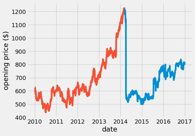
I only want the symbol == GOOGL data, so I use a Pandas call. I also want to remove the big drop in price after Mar, 2014, so I specify the date < 2014-03-01.

google_data = data[data['symbol'] == 'GOOGL']

plt.plot(google_data['date'], google_data['open'])

# remove data > 2014-03-01

google_data_pre_2014 = google_data[ google_data['date'] < pd.to_datetime('2014-03-01')]
plt.plot(google_data_pre_2014['date'], google_data_pre_2014['open'])
plt.xlabel('date')
plt.ylabel('opening price (\$)');

2. Data analysis#

The GOOGL stock nearly doubled in price from 2010 through 2014. Day-to-day, the price fluctuates randomly. Here, I look at the fluctuations in price using np.diff.

dprice = np.diff(google_data_pre_2014['open'])
plt.plot(google_data_pre_2014['date'][1:], dprice)
plt.xlabel('date')
plt.ylabel('change in opening price (\$/day)');

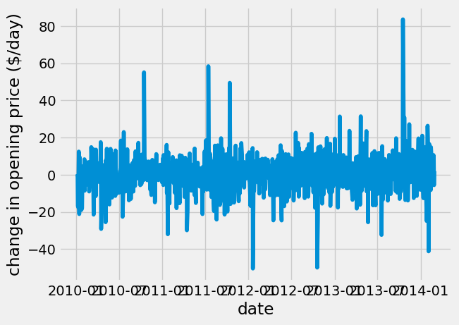
Looking at the price day-to-day, it would appear to be an average change of $0/day. Next, I explore the statistical results of the change in opening price

mean
standard deviation
histogram

mean_dprice = np.mean(dprice)
std_dprice = np.std(dprice)
x = np.linspace(-40, 40)
from scipy import stats
price_pdf = stats.norm.pdf(x, loc = mean_dprice, scale = std_dprice)

plt.hist(dprice, 50, density=True)
plt.plot(x, price_pdf)
plt.title('GOOGL changes in price over 4 years\n'+
         'avg: \${:.2f} stdev: \${:.2f}'.format(mean_dprice, std_dprice));

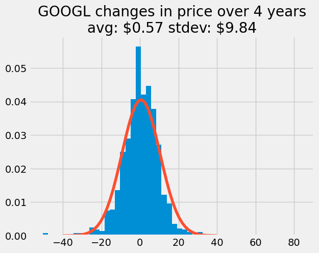
From this statistical result, it looks like the price changes followed a normal distribution with an average change of $\$0.57$ and a standard deviation of $\$9.84$.

3. Create random variables#

Now, I know the distribution shape and characteristics to simulate the random walk price changes for the GOOGL prices each day. Here, I generate random variables with the following array structure:

Date	model 1	model 2	model 3	…	model N
day 1	$\Delta \$ model~1$	$\Delta \$ model~2$	$\Delta \$ model~3$	…	$\Delta \$ model~N$
day 2	$\Delta \$ model~1$	$\Delta \$ model~2$	$\Delta \$ model~3$	…	$\Delta \$ model~N$
…	…	…	…	…	…

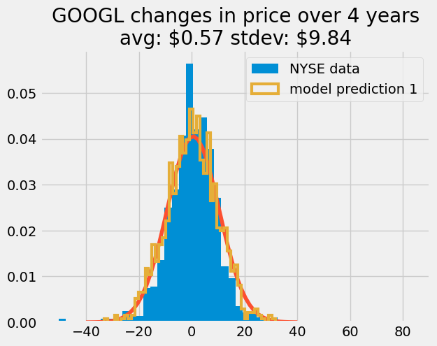
Each column is one random walk model. Each row is one simulated day. If I want to look at one model predition, I would plot one column. If I want to look at the average result, I take the average of each row. To start, I’ll create 100 random walk models. I use the normal distribution to match the statistical distribution I found in part 2.

rng = default_rng(42)
N_models = 100
dprice_model = rng.normal(size = (len(google_data_pre_2014), N_models), loc = 0.568, scale = 9.838)

plt.hist(dprice, 50, density=True, label = 'NYSE data')
plt.plot(x, price_pdf)
plt.hist(dprice_model[:, 0], 50, density = True, 
         histtype = 'step', 
         linewidth = 3, label = 'model prediction 1')
plt.title('GOOGL changes in price over 4 years\n'+
         'avg: \${:.2f} stdev: \${:.2f}'.format(mean_dprice, std_dprice))
plt.legend();

4. Generate random walk predictions#

Above, I show tha the simulated data follows the requested normal distribution. Now, I can cumulatively sum these steps to predict the stock prices each day. I use the np.cumsum argument, axis = 0 to sum along the columns i.e. each row becomes the sum of previous rows.

>>> a = np.array([[1,2,3], [4,5,6]])
>>> a
array([[1, 2, 3],
       [4, 5, 6]])
>>>> np.cumsum(a,axis=0)      # sum over rows for each of the 3 columns
array([[1, 2, 3],
       [5, 7, 9]])

Then, I plot all of the random walk models to compare to the NYSE data. The models are given transparency using the alpha = 0.3 command (alpha = 0 is invisible, alpha = 1 is opaque).

price_model = np.cumsum(dprice_model, axis = 0) + google_data_pre_2014['open'].values[0]

plt.plot(google_data_pre_2014['date'], price_model, alpha = 0.3);

plt.plot(google_data_pre_2014['date'], google_data_pre_2014['open'], c = 'k', label = 'NYSE data')
plt.xlabel('date')
plt.ylabel('opening price (\$)');

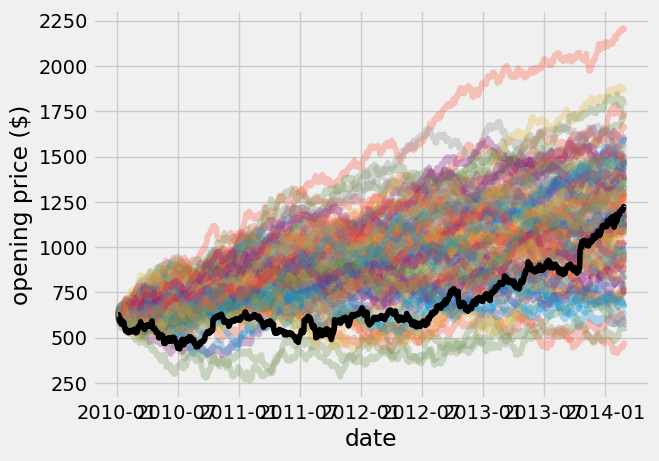
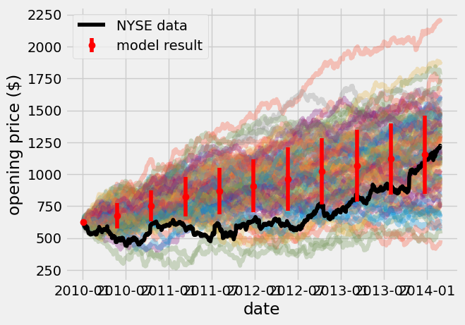
As you would expect, there are a wide variety of predictions for the price of GOOGL stocks using random numbers. Next, I try to get some insight into the average changes in the random walk model. I use the np.mean and np.std across the columns of the price_model prediction data, using axis = 1 now.

price_model_avg = np.mean(price_model, axis = 1)
price_model_std = np.std(price_model, axis = 1)

plt.plot(google_data_pre_2014['date'], price_model, alpha = 0.3);

plt.plot(google_data_pre_2014['date'], google_data_pre_2014['open'], c = 'k', label = 'NYSE data')
plt.xlabel('date')
plt.ylabel('opening price (\$)');

skip = 100
plt.errorbar(google_data_pre_2014['date'][::skip], price_model_avg[::skip],
             yerr = price_model_std[::skip], 
             fmt = 'o',
             c = 'r', 
             label = 'model result', 
            zorder = 3);
plt.legend();
    

Wrapping up#

In this analysis, I went through data exploration, analysis, and Monte Carlo model prediction. The average random walk should resemble a straight line. There are further insights you can get by analyzing the random walk data, but for now it looks like we can accurately predict the growth of GOOGL stock over four years. What are some caveats to this method? If we continue to predict prices into 2015, what would happen compared to the real data?

Next Steps#

Now, you can try your hand at predicting stock prices on your own stock. Choose your own stock symbol and go through the same 4 steps I detailed above:

Explore data and select your own stock of interest
Find statistical description of data: mean and standard deviation _use some of the graphing + analysis techniques in 01_Cheers_stats_beers and 02_Seeing_stats.
Create random variables
Generate random walk for choose your own stock opening price

Here are the list of stocks in this dataset: ‘A’, ‘AAL’, ‘AAP’, ‘AAPL’, ‘ABBV’, ‘ABC’, ‘ABT’, ‘ACN’, ‘ADBE’, ‘ADI’, ‘ADM’, ‘ADP’, ‘ADS’, ‘ADSK’, ‘AEE’, ‘AEP’, ‘AES’, ‘AET’, ‘AFL’, ‘AGN’, ‘AIG’, ‘AIV’, ‘AIZ’, ‘AJG’, ‘AKAM’, ‘ALB’, ‘ALK’, ‘ALL’, ‘ALLE’, ‘ALXN’, ‘AMAT’, ‘AME’, ‘AMG’, ‘AMGN’, ‘AMP’, ‘AMT’, ‘AMZN’, ‘AN’, ‘ANTM’, ‘AON’, ‘APA’, ‘APC’, ‘APD’, ‘APH’, ‘ARNC’, ‘ATVI’, ‘AVB’, ‘AVGO’, ‘AVY’, ‘AWK’, ‘AXP’, ‘AYI’, ‘AZO’, ‘BA’, ‘BAC’, ‘BAX’, ‘BBBY’, ‘BBT’, ‘BBY’, ‘BCR’, ‘BDX’, ‘BEN’, ‘BHI’, ‘BIIB’, ‘BK’, ‘BLK’, ‘BLL’, ‘BMY’, ‘BSX’, ‘BWA’, ‘BXP’, ‘C’, ‘CA’, ‘CAG’, ‘CAH’, ‘CAT’, ‘CB’, ‘CBG’, ‘CBS’, ‘CCI’, ‘CCL’, ‘CELG’, ‘CERN’, ‘CF’, ‘CFG’, ‘CHD’, ‘CHK’, ‘CHRW’, ‘CHTR’, ‘CI’, ‘CINF’, ‘CL’, ‘CLX’, ‘CMA’, ‘CMCSA’, ‘CME’, ‘CMG’, ‘CMI’, ‘CMS’, ‘CNC’, ‘CNP’, ‘COF’, ‘COG’, ‘COH’, ‘COL’, ‘COO’, ‘COP’, ‘COST’, ‘COTY’, ‘CPB’, ‘CRM’, ‘CSCO’, ‘CSRA’, ‘CSX’, ‘CTAS’, ‘CTL’, ‘CTSH’, ‘CTXS’, ‘CVS’, ‘CVX’, ‘CXO’, ‘D’, ‘DAL’, ‘DD’, ‘DE’, ‘DFS’, ‘DG’, ‘DGX’, ‘DHI’, ‘DHR’, ‘DIS’, ‘DISCA’, ‘DISCK’, ‘DLPH’, ‘DLR’, ‘DLTR’, ‘DNB’, ‘DOV’, ‘DOW’, ‘DPS’, ‘DRI’, ‘DTE’, ‘DUK’, ‘DVA’, ‘DVN’, ‘EA’, ‘EBAY’, ‘ECL’, ‘ED’, ‘EFX’, ‘EIX’, ‘EL’, ‘EMN’, ‘EMR’, ‘ENDP’, ‘EOG’, ‘EQIX’, ‘EQR’, ‘EQT’, ‘ES’, ‘ESRX’, ‘ESS’, ‘ETFC’, ‘ETN’, ‘ETR’, ‘EVHC’, ‘EW’, ‘EXC’, ‘EXPD’, ‘EXPE’, ‘EXR’, ‘F’, ‘FAST’, ‘FB’, ‘FBHS’, ‘FCX’, ‘FDX’, ‘FE’, ‘FFIV’, ‘FIS’, ‘FISV’, ‘FITB’, ‘FL’, ‘FLIR’, ‘FLR’, ‘FLS’, ‘FMC’, ‘FOX’, ‘FOXA’, ‘FRT’, ‘FSLR’, ‘FTI’, ‘FTR’, ‘FTV’, ‘GD’, ‘GE’, ‘GGP’, ‘GILD’, ‘GIS’, ‘GLW’, ‘GM’, ‘GOOG’, ‘GOOGL’, ‘GPC’, ‘GPN’, ‘GPS’, ‘GRMN’, ‘GS’, ‘GT’, ‘GWW’, ‘HAL’, ‘HAR’, ‘HAS’, ‘HBAN’, ‘HBI’, ‘HCA’, ‘HCN’, ‘HCP’, ‘HD’, ‘HES’, ‘HIG’, ‘HOG’, ‘HOLX’, ‘HON’, ‘HP’, ‘HPE’, ‘HPQ’, ‘HRB’, ‘HRL’, ‘HRS’, ‘HSIC’, ‘HST’, ‘HSY’, ‘HUM’, ‘IBM’, ‘ICE’, ‘IDXX’, ‘IFF’, ‘ILMN’, ‘INTC’, ‘INTU’, ‘IP’, ‘IPG’, ‘IR’, ‘IRM’, ‘ISRG’, ‘ITW’, ‘IVZ’, ‘JBHT’, ‘JCI’, ‘JEC’, ‘JNJ’, ‘JNPR’, ‘JPM’, ‘JWN’, ‘K’, ‘KEY’, ‘KHC’, ‘KIM’, ‘KLAC’, ‘KMB’, ‘KMI’, ‘KMX’, ‘KO’, ‘KORS’, ‘KR’, ‘KSS’, ‘KSU’, ‘L’, ‘LB’, ‘LEG’, ‘LEN’, ‘LH’, ‘LKQ’, ‘LLL’, ‘LLTC’, ‘LLY’, ‘LMT’, ‘LNC’, ‘LNT’, ‘LOW’, ‘LRCX’, ‘LUK’, ‘LUV’, ‘LVLT’, ‘LYB’, ‘M’, ‘MA’, ‘MAA’, ‘MAC’, ‘MAR’, ‘MAS’, ‘MAT’, ‘MCD’, ‘MCHP’, ‘MCK’, ‘MCO’, ‘MDLZ’, ‘MDT’, ‘MET’, ‘MHK’, ‘MJN’, ‘MKC’, ‘MLM’, ‘MMC’, ‘MMM’, ‘MNK’, ‘MNST’, ‘MO’, ‘MON’, ‘MOS’, ‘MPC’, ‘MRK’, ‘MRO’, ‘MSFT’, ‘MSI’, ‘MTB’, ‘MTD’, ‘MU’, ‘MUR’, ‘MYL’, ‘NAVI’, ‘NBL’, ‘NDAQ’, ‘NEE’, ‘NEM’, ‘NFLX’, ‘NFX’, ‘NI’, ‘NKE’, ‘NLSN’, ‘NOC’, ‘NOV’, ‘NRG’, ‘NSC’, ‘NTAP’, ‘NTRS’, ‘NUE’, ‘NVDA’, ‘NWL’, ‘NWS’, ‘NWSA’, ‘O’, ‘OKE’, ‘OMC’, ‘ORCL’, ‘ORLY’, ‘OXY’, ‘PAYX’, ‘PBCT’, ‘PBI’, ‘PCAR’, ‘PCG’, ‘PCLN’, ‘PDCO’, ‘PEG’, ‘PEP’, ‘PFE’, ‘PFG’, ‘PG’, ‘PGR’, ‘PH’, ‘PHM’, ‘PKI’, ‘PLD’, ‘PM’, ‘PNC’, ‘PNR’, ‘PNW’, ‘PPG’, ‘PPL’, ‘PRGO’, ‘PRU’, ‘PSA’, ‘PSX’, ‘PVH’, ‘PWR’, ‘PX’, ‘PXD’, ‘PYPL’, ‘QCOM’, ‘QRVO’, ‘R’, ‘RAI’, ‘RCL’, ‘REGN’, ‘RF’, ‘RHI’, ‘RHT’, ‘RIG’, ‘RL’, ‘ROK’, ‘ROP’, ‘ROST’, ‘RRC’, ‘RSG’, ‘RTN’, ‘SBUX’, ‘SCG’, ‘SCHW’, ‘SE’, ‘SEE’, ‘SHW’, ‘SIG’, ‘SJM’, ‘SLB’, ‘SLG’, ‘SNA’, ‘SNI’, ‘SO’, ‘SPG’, ‘SPGI’, ‘SPLS’, ‘SRCL’, ‘SRE’, ‘STI’, ‘STT’, ‘STX’, ‘STZ’, ‘SWK’, ‘SWKS’, ‘SWN’, ‘SYF’, ‘SYK’, ‘SYMC’, ‘SYY’, ‘T’, ‘TAP’, ‘TDC’, ‘TDG’, ‘TEL’, ‘TGNA’, ‘TGT’, ‘TIF’, ‘TJX’, ‘TMK’, ‘TMO’, ‘TRIP’, ‘TROW’, ‘TRV’, ‘TSCO’, ‘TSN’, ‘TSO’, ‘TSS’, ‘TWX’, ‘TXN’, ‘TXT’, ‘UAA’, ‘UAL’, ‘UDR’, ‘UHS’, ‘ULTA’, ‘UNH’, ‘UNM’, ‘UNP’, ‘UPS’, ‘URBN’, ‘URI’, ‘USB’, ‘UTX’, ‘V’, ‘VAR’, ‘VFC’, ‘VIAB’, ‘VLO’, ‘VMC’, ‘VNO’, ‘VRSK’, ‘VRSN’, ‘VRTX’, ‘VTR’, ‘VZ’, ‘WAT’, ‘WBA’, ‘WDC’, ‘WEC’, ‘WFC’, ‘WFM’, ‘WHR’, ‘WLTW’, ‘WM’, ‘WMB’, ‘WMT’, ‘WRK’, ‘WU’, ‘WY’, ‘WYN’, ‘WYNN’, ‘XEC’, ‘XEL’, ‘XL’, ‘XLNX’, ‘XOM’, ‘XRAY’, ‘XRX’, ‘XYL’, ‘YHOO’, ‘YUM’, ‘ZBH’, ‘ZION’, ‘ZTS’

Date	model 1	model 2	model 3	…	model N
day 1	\(\Delta \$ model~1\)	\(\Delta \$ model~2\)	\(\Delta \$ model~3\)	…	\(\Delta \$ model~N\)
day 2	\(\Delta \$ model~1\)	\(\Delta \$ model~2\)	\(\Delta \$ model~3\)	…	\(\Delta \$ model~N\)
…	…	…	…	…	…