
Wind Turbine Uncertainty in loading analysis#
James Arnold#
Abstract#
The design and analysis of wind turbines involves significant uncertainties in materials, loads, and structural performance. These uncertainties can affect the reliability and efficiency of wind turbines, requiring methods to address this uncertainty. Monte Carlo simulation is a statistical tool used to address these uncertainties. This report explores the application of Monte Carlo simulation to assess the uncertainties in materials, loads, and structural performance of wind turbines. This report will feature a study examining the difference in the stress distribution and power output of a wind turbine blade at a length of 40 meters and 50 meters. The study demonstrates how Monte Carlo methods can enhance the understanding and management of these uncertainties, ultimately contributing to more reliable and efficient wind turbine designs.
import numpy as np
import scipy.stats as stats
import matplotlib.pyplot as plt
I. Introduction#
Wind turbines use blades to collect the wind’s kinetic energy. Wind flows over the blades creating lift which causes the blades to turn. The blades are connected to a drive shaft that turns an electric generator, which produces electricity. Wind electricity generation has grown significantly in the past 30 years. The three major components of a wind turbine are a rotor, nacelle, and tower. The rotor consists of a hub and three blades [1]. The hub is the link between the blades and shaft. The blades obtain kinetic energy from the wind. This is converted to torque and transferred to the gearbox through the shaft [1]. To maximize energy capture, the turbine rotates on its vertical axis to position the rotor in the direction of the wind using a yawning mechanism. The major components in the nacelle include the gearbox and generator [1]. The rotor and gearbox are connected using a low-speed shaft. The gearbox and generator are connected using a high-speed shaft. The rotation of the blades converts a low-speed, high-torque to a high-speed, low-torque rotational force transferred to the generator using the gearbox. The tower is connected to the ground and the rotor and nacelle are connected to the top of the tower [1]. The tower is typically 262-360 feet [1]. The types of uncertainty in wind turbine design include aleatoric and epistemic uncertainty. Aleatoric uncertainty if fixed and includes uncertainty in due to turbulence and material yield/fatigue stress [7]. This also includes uncertainty in the environment and loads the structure experiences [6]. These uncertainties require probabilistic mathematical methods to understand the uncertainty involved [6]. Epistemic uncertainty is reducible and includes uncertainty in site condition parameters and aerodynamic models [7]. Wind turbines utilize many different materials. Steel is often used in the tower and nacelle as it has a high tensile strength and durability. Fiberglass and carbon fiber composites are often used for blades as they have a high strength-to-weight ratio [3]. Aluminum is often used for some components because of its lightweight properties and corrosion resistance. The materials go through different manufacturing processes which leads to differences in material properties. Environmental exposure such as UV radiation, moisture, temperature fluctuations and salt sprayed in offshore turbines affect the material strength over time [3]. Additionally, fatigue cycles are impacted by load cycles, geometry, and operational conditions [4]. Stress concentration and magnitude of load cycles greatly impact the fatigue cycles of the materials in wind turbines [4]. Weibull distribution is often used to accurately estimate energy production and wind speed. Weibull distribution is commonly used as it predicts wind conditions and inverse of wind direction [5]. Weibull distribution uses wind speed and shape parameters to create a probability function. Modelling Weibull distribution can help accurately estimate uncertainty. Weibull distribution is effective for calculating probability of failure. Monte Carlo simulations are often used to address uncertainty in wind turbine design [5]. Monte Carlo is the most simple sampling technique. Monte Carlo methods use random sampling to create a probability distribution. Monte Carlo simulations are often used to obtain wind turbine output power at each hour [5]. Using Monte Carlo methods, the input variables are modelled with associated uncertainty and address the cumulative impact on the variables outputted [5]. Monte Carlo simulations are simple and easier to develop but often other methods produce more accurate results.
II. Sources of Uncertainty in Wind Turbine Design#
Wind turbine design has a significant amount of uncertainty associated with it. Wind turbines utilize many different materials. Steel is often used in the tower and nacelle as it has a high tensile strength and durability. Steel is used for structural loads as it is a high-strength material especially in tension. Steel is durable and versatile however, it has poor corrosion resistance which can cause uncertainty and decrease reliability. Additionally, steel has strong thermal conductivity which can complicate heating, cooling and insulation of structures made of steel. Steel has good fatigue strength, so it can withstand a higher magnitude of stress than alternate materials considered for use. Fiberglass and carbon fiber composites are often used for blades as they have a high strength-to-weight ratio. Fiberglass is lightweight yet is often stronger than other metals such as steel. Fiberglass is non-conductive and durable making it sustainable. Fiberglass can degrade over time when it is exposed to prolonged sunlight or other weather conditions. This adds uncertainty to the system as fiberglass might not be able to be used for long term use such as wind turbine design. Lifetime constraints must be considered for uncertainty in wind turbine design. Aluminum is often used for some components because of its lightweight properties and corrosion resistance. Aluminum has a low density and has excellent thermal conductivity which makes it a desirable material for design. Aluminum is also an excellent reflector of radiant energy, has a high electrical conductivity and is resistant to corrosion. Aluminum has a low tensile strength compared to other metals. This adds uncertainty as aluminum has constraints for the amount of loading that it can handle. The materials considered during the design process go through different manufacturing processes. As a result, each material has different tolerancing restrictions and uncertainty is added through each tolerance and constraint involved. Environmental exposure such as UV radiation, moisture, temperature fluctuations and salt sprayed in offshore turbines affect the material strength over time. Fatigue cycles are impacted by load cycles, geometry, and operational conditions. Stress concentration and magnitude of load cycles greatly impact the fatigue cycles of the materials in wind turbines.
Various loads are applied onto different components of wind turbines. Wind turbine blades experience aerodynamic, gravitational and inertial loads [2]. Aerodynamic loads are due to wind pushing up against the blades. This load is proportional to the wind speed and the area of the blade. Gravitational loads are due to the weight of the blade [2]. Inertial load is due to rotational motion of the blades, particularly during changes in rotational speed or direction. Each load adds uncertainty to the system [2]. Wind turbines experience heavy loads which adds a significant degree of uncertainty to wind turbines. Geometry of wind turbine is an important consideration. Power production of a wind turbine blade increases as the area of the blade increases. Increasing blade area increases uncertainty. Understanding uncertainty in the geometry of a turbine blade produces a more efficient blade design. Several methods are available for use to address the uncertainty involved in wind turbine design.
III. Methods to Address Uncertainty#
Monte Carlo simulations are often used to address uncertainty in wind turbine design. Monte Carlo is the most simple sampling technique. Monte Carlo methods use random sampling to create a probability distribution. Monte Carlo simulations are often used to obtain wind turbine output power at each hour. Using Monte Carlo methods, the input variables are modelled with associated uncertainty and address the cumulative impact on the variables outputted. Monte Carlo simulations are simple and easier to develop but often other methods produce more accurate results. Weibull distribution is often used to accurately estimate power production and wind speed. Weibull distribution is commonly used as it predicts wind conditions and inverse of wind direction. Weibull distribution uses wind speed and shape parameters to create a probability function. Modelling Weibull distribution can help accurately estimate uncertainty.
This study focuses on the difference in stress and power production between wind turbine blades with a length of 40 meters and 50 meters. This study is an example of using Monte Carlo methods to simulate uncertainty of materials, loads and structures in wind turbine design is shown below. Pseudo-random number generators are used in the simulation to create random samples for each uncertain parameter according to their probability distributions. The simulation is run to form a distribution of the outcome. The blade is assumed to be made out of fiberglass. The fiberglass is assumed to have a Young’s Modulus of 70 GPa with a standard deviation of 5 GPa.
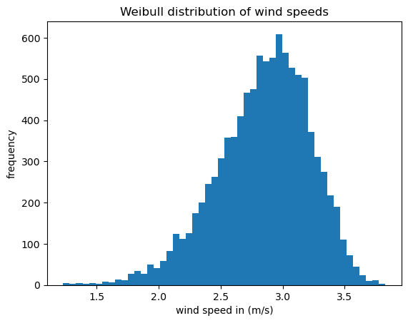
The wind speed is assumed to follow a Weibull distribution with a shape parameter of k = 9 and a scale parameter of 3. The resulting distribution is shown below in the “Weibull distribution of wind speeds”. The average wind speed is 2.8 m/s with a standard deviation of 0.4 m/s.
num_simulations = 10000
# Material properties (Young's modulus in GPa)
E_mean = 70
E_std = 5
E_samples = np.random.normal(E_mean, E_std, num_simulations)
# Wind speed (m/s)
k = 9
lam = 3
wind_speed_samples = np.random.weibull(k, num_simulations) * lam

plt.hist(wind_speed_samples, 50)
plt.title('Weibull distribution of wind speeds')
plt.xlabel('wind speed in (m/s)')
plt.ylabel('frequency')
print(wind_speed_samples.mean(), wind_speed_samples.std())
2.8461940171445894 0.3764522177570118
The length of the blade is assumed to be 40 m with a standard deviation of 0.1 m in the first simulation. The second simulation assumes the length of the blade to be 50 meters with a standard deviation of 0.1 m. The formula for the stress of the blade is:
\(\sigma_{b,~max} = \frac{Mc}{I_c} = \frac{F_D L^2}{2}\frac{c}{I_c}\) (1)
where v is the wind speed velocity, E is the Young’s modulus value, and L is the length of the blade.
The formula for the power output of the wind turbine blade is:
\(P = 0.5 \rho A_{turbine} v^{3} c_{p}\) (2)
where P is the power output, ρ is the air density which is 1.225 kg/m^3^, \(A_{turbine}\) is the turbine blade swept area, and \(c_p\) is the power coefficient. The power coefficient is 0.4 for this simulation. The code and results of the simulation is provided below:
# Blade length (m)
w = 2 # width of blade
t = 0.5 # thickness of blade
c = t/2 # centroidal distance
I = w*t**3/12
Cd = 0.5 # drag coefficient
rho = 1 # kg/m^3 density of air
for L_mean in [40, 50]:
    L_std = 0.1
    L_samples = np.random.normal(L_mean, L_std, num_simulations)
    # Placeholder for results
    stress_samples = []
    Power_samples = []
    # Perform simulations
    for i in range(num_simulations):
        E = E_samples[i]
        V = wind_speed_samples[i]
        L = L_samples[i]
        # Simplified stress calculation (example)
        # Stress = function(E, V, L)
        stress = (0.5 *Cd*rho* V**2)*L**2/2*c/I # Simplified example
        stress_samples.append(stress)
        # Power Output in MW

        # Air Density in kg/m^3
        den = 1.225
        # Area of the Turbine Swept
        A = 3.14 * L**2
        Power = 0.5 * den * A * V * 0.4
        Power_samples.append(Power)
    # Convert results to a NumPy array
    stress_samples = np.array(stress_samples)
    # Convert results to a NumPy array
    Power_samples = np.array(Power_samples)


    # Analyze results
    mean_stress = np.mean(stress_samples)
    std_stress = np.std(stress_samples)
    Power_result = np.mean(Power_samples)
    # Print results
    print(f"Mean Stress at {L_mean} meters: {mean_stress:.5f} Pa")
    print(f"Standard Deviation of Stress at {L_mean} meters: {std_stress:.5f} Pa")
    print(f"Power at {L_mean} meters: {Power_result:.5f} W")

    # Plot results
    plt.figure(1)
    plt.hist(stress_samples/1e6,
             bins=50,
             density=True,
             alpha=0.6,
            label = 'length = {:0.0f} m'.format(L))#, color='g')
    plt.title('Histogram of Stress Distribution')
    plt.xlabel('Stress (MPa)')
    plt.ylabel('Frequency')
    plt.legend();

    plt.figure(2)
    plt.hist(Power_samples,
             bins=50,
             density=True,
             alpha=0.6,
            label = 'length = {:0.0f} m'.format(L))#, color='g')
    plt.title('Histogram of Power outputs for wind speeds')
    plt.xlabel('Power (MW)')
    plt.ylabel('Frequency')
    plt.legend();
    plt.figure(3)
    plt.plot(stress_samples/1e6, Power_samples, 's',
             label = 'length = {:0.0f} m'.format(L))
    plt.title('relation between power and max stress')
    plt.ylabel('Power (MW)')
    plt.xlabel('Stress (MPa)')
    plt.legend();
Mean Stress at 40 meters: 19781.57596 Pa
Standard Deviation of Stress at 40 meters: 4981.54793 Pa
Power at 40 meters: 3503.23805 W
Mean Stress at 50 meters: 30910.68075 Pa
Standard Deviation of Stress at 50 meters: 7786.16776 Pa
Power at 50 meters: 5474.08402 W
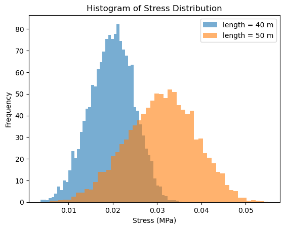
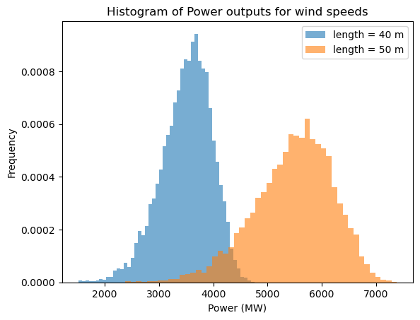
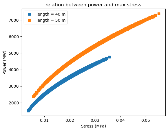
Figure 1: Stress results for turbine blades of 40-m and 50-m and below are the power outputs comparing the 40-m and 50-m turbine blades.
Figure 2: The Mean Stress, Standard Deviation of Stress, and Histogram of the Stress Distribution of the Monte Carlo Simulation and the Power Developed By the Turbine Blade of the Wind Turbine With a Length of 40 and 50 Meters
Figure 3: There is a correlation between max stress and power output due to the combined loading of lift and drag on the wind turbine blades. The 50-m blades have higher power and higher stress as wind speeds increase.
This figure shows that mean stress on the wind turbine blade is 0.00147 Pa while the standard deviation is 0.00038 Pa for a blade with a length of 40 meters. The power developed by the turbine blade is 3038.90 W. The shape of the histogram of the stress distribution of the turbine blade is as expected. The middle of the blade experiences more stress than the edges so the most stress is applied at the halfway point of the length on the blade.
This figure shows that mean stress on the wind turbine blade is 0.00118 Pa while the standard deviation is 0.00031 Pa for a blade with a length of 50 meters. The power developed by the turbine blade is 4753.36 W. The shape of the histogram of the stress distribution of the turbine blade is as expected. The middle of the blade experiences more stress than the edges so the most stress is applied at the halfway point of the length on the blade.
The Monte Carlo simulations are often used to address uncertainty in wind turbine design. Monte Carlo is the most simple sampling technique. Monte Carlo methods use random sampling to create a probability distribution. Monte Carlo simulations are often used to obtain wind turbine output power at each hour. Using Monte Carlo methods, the input variables are modelled with associated uncertainty and address the cumulative impact on the variables outputted. Monte Carlo simulations are simple and easier to develop but often other methods produce more accurate results.
Miner’s rules is used to plot the number of cycles to failure to the stress applied. Miner’s rule is often used in fatigue analysis. The code output of Miner’s rule is:
lifetime = 10**np.array([4,5,6,7,8,9])
stress = np.array([43,32,25,20,16,14])
plt.semilogy(stress*6.89476, lifetime)
plt.semilogy(stress*6.89476,
            10**np.interp(stress*6.89476, stress*6.89476, np.log10(lifetime)))
plt.xlabel('Stress (MPa)')
plt.ylabel('Number of Cycles')
Text(0, 0.5, 'Number of Cycles')
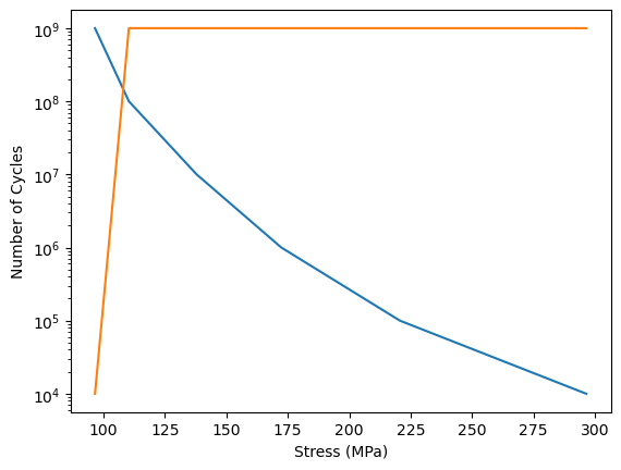
Figure 3: Code and Output Using Miner’s Rule
This figure shows that the number of cycles before failure is 10^9. The selected material can endure loading for a long period of time as this turbine blades endure in this simulation. This means that the selected material is reliable. Fiberglass was a good material to be selected as it is reliable and can endure the applied load. The turbine blades can survive the load applied by the wind.
IV. Conclusion#
This case study focused on the difference in stress and power production between wind turbine blades with a length of 40 meters and 50 meters. This study is an example of using Monte Carlo methods to simulate uncertainty of materials, loads and structures in wind turbine design. Pseudo-random number generators are used in the simulation to create random samples for each uncertain parameter according to their probability distributions. The simulation is run to form a distribution of the outcome. The mean stress on the wind turbine blade with a length of 40 meters is 0.00147 Pa while the standard deviation is 0.00038 Pa. The power developed by the turbine blade is 3038.90 W. The mean stress on the wind turbine blade with a length of 50 meters is 0.00118 Pa while the standard deviation is 0.00031 Pa. The power developed by the turbine blade is 4753.36 W.
This study validates the idea that with increasing length on turbine blades the stress decreases. The 50-meter blade endured four ten-thousands Pa less than the 40-meter blade. Both simulations outputted the same standard deviation of stress. The range of the stress distribution was roughly the same, however the 40-meter blade is subject to more stress. This can reduce the sustainability of the blade. This study proved that stress of a wind turbine blade decreases when the length increases.
This study validated that the longer the turbine blade, the more power will be produced. The 50-meter blade produced 1714.46 W more than the 40-meter blade. The power production of the second simulation was substantially greater than the first simulation. Power production increased as the area of the turbine swept increased. The area increased significantly in the second simulation due to the blade being 10 meters longer, which increased the power production by the blade. The wind speed remained constant for both experiments, proving that the increased area contributed to the higher power production. This study proved that power production of a wind turbine blade increases when the length increases. Additionally, this study showed that the number of cycles before failure is 10^9^. This means that the material is reliable. The turbine blades can survive the load applied by the wind.
Stress distribution and power production are important considerations for wind turbine blades however other considerations are needed. Sourcing a longer blade requires financial considerations as well as efficiency considerations. Longer blades require more material, increasing product cost. Each project has a budget and requiring more material can exceed budget limits. Additionally, longer blades create more concerns and uncertainties. Longer blades increase vibrations and require complex control requirements. Designing longer blades can be impractical as the blades become heavier. Uncertainty increases with longer blades. Wind turbine blades 50 meters long are the perfect length. Stress and power production are optimized, and uncertainty is simpler. Blades 60 meters or longer produce higher uncertainties and are often impractical. Blades 50 meters in length produce high power production while maintaining a low stress distribution. This study proved that a 50-meter turbine blade produces more power and less stress than a 40-meter blade. Understanding uncertainties in wind turbine blade design helps examine how to efficiently design a wind turbine blade.
V. References#
“How a Wind Turbine Works - Text Version | Department of Energy.” Wind Energy Technologies Office, Office of Energy Efficiency & Renewable Energy, www.energy.gov/eere/wind/how-wind-turbine-works-text-version. Accessed 21 June 2024.
Madsen, Peter. Predicting Ultimate Loads for Wind Turbine Design, National Renewable Energy Labratory, Nov. 1998, www.nrel.gov/docs/fy99osti/25787.pdf.
Murphy, Patrick, et al. “How Wind Speed Shear and Directional Veer Affect the Power Production of a Megawatt-Scale Operational Wind Turbine.” Wind Earth Science, European Academy of Wind Energy, 11 Sept. 2020, www.nrel.gov/docs/fy20osti/78107.pdf.
Nijssen, R.P.L. “Fatigue Life Prediction and Strength Degradation of Wind Turbine Rotor Blade Composites.” Unlimited Release, Sandia, Oct. 2007, energy.sandia.gov/wp-content/gallery/uploads/SAND-2006-7810p.pdf.
Sanderse, Benjamn. Uncertainty Quantification for Wind Energy Applications - Literature Review, Research Gate, Aug. 2017, www.researchgate.net/publication/319209260_Uncertainty_quantification_for_wind_energy_applications_-_Literature_review.
Stieng, Lars Einar S., and Michael Muskulus. “Reliability-Based Design Optimization of Offshore Wind Turbine Support Structures Using Analytical Sensitivities and Factorized Uncertainty Modeling.” Wind Energy Science, Copernicus GmbH, 29 Jan. 2020, wes.copernicus.org/articles/5/171/2020/.
Witcher, David. “Uncertainty Quantification Techniques in Wind Turbine Design.” DNV GL – RENEWABLES ADVISORY , DNV-GL, www.nrel.gov/wind/assets/pdfs/se17-2-uncertainty-in-wind-turbine-design-process.pdf. Accessed 22 June 2024.