import numpy as np
import matplotlib.pyplot as plt
from numpy.random import default_rng
plt.style.use('fivethirtyeight')
Statistical Significance in Data#
How many measurements do you need to prove two measurements are different?
This is a problem of constant debate with many different approaches,
In all of these approaches, scientists and engineers create a quantitative test to accept or reject the hypothesis that two set of data are not significantly different. This concept was very strange to me at first. How can two different measurements be considered the same? It wasn’t until I started practicing, building, and applying engineering concepts that this question started to make sense.
Generate some data we know is different#
Monte Carlo experiments are a great way to start understanding this difficult question, lets build x2 100-value data sets. Consider a case where two people, Pat and Jim, are going to throw the same size ball as far as possible. We know Pat is stronger than Jim. Pat creates an average of 68 J of work throwing a ball, and Jim creates an average of 65 J.
Pat is on average \(\frac{38 - 35}{35} = \frac{3}{35} = 8.6\%\) stronger than Jim. Let’s assume both Pat and Jim can sometimes throw a little faster and sometimes a little slower so the actual values are \(68\pm 3~J\) and \(65\pm 2~J\). Now, we have a statistical comparison
normal distribution at \(38 \pm 3~J\)
normal distribution at \(35 \pm 2~J\)
rng = default_rng(42)

Pat = rng.normal(loc = 38, scale = 3, size = 100)
Jim = rng.normal(loc = 35, scale = 2, size = 100)

plt.hist(Pat,
        histtype='step',
        linewidth = 4,
         label = 'Pat',
         density = True,)
        #bins = np.linspace(50,80, 31))
plt.hist(Jim,
        histtype = 'step',
        linewidth = 4,
         label = 'Jim',
         density = True,)
        #bins =np.linspace(50, 80, 41))
plt.xlabel('avg work of throw')
plt.ylabel('relative number of throws')
plt.legend();
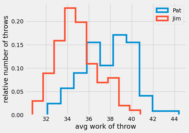
print('set01 = {:1.2f} +/- {:1.2f}'.format(np.mean(Pat), np.std(Pat)))
print('set02 = {:1.2f} +/- {:1.2f}'.format(np.mean(Jim), np.std(Jim)))
set01 = 37.85 +/- 2.32
set02 = 34.98 +/- 1.95
Are these measurements different?#
The two histograms are different, but many of the values throws between Pat and Jim are the same. For example, both throwers had work of 66 J 10-15% of the throws. If we only consider the reported means, 67.9 and 65, there is a significant difference between the two results, but how accurate is this value of mean?
Lets calculate more data sets and see how much the much the mean can change.
set_01 = rng.normal(loc = 38, scale = 3, size = (50, 100))
set_02 = rng.normal(loc = 35, scale = 2, size = (50, 100))
mean_01 = np.mean(set_01, axis = 1)
mean_02 = np.mean(set_02, axis = 1)
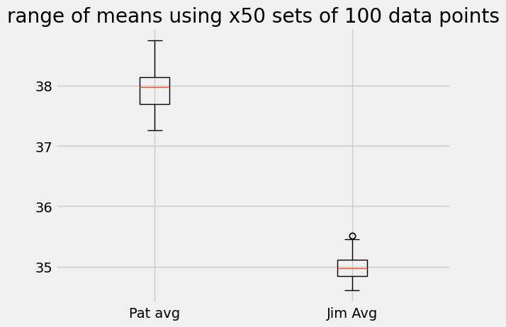
plt.boxplot([mean_01, mean_02], labels=['Pat avg', 'Jim Avg'])
plt.title('range of means using x50 sets of 100 data points')
Text(0.5, 1.0, 'range of means using x50 sets of 100 data points')
plt.hist(mean_01,
        histtype='step',
        linewidth = 4,)
        #bins = np.linspace(-0.5,1.5, 31))
plt.hist(mean_02,
        histtype = 'step',
        linewidth = 4,)
        #bins =np.linspace(-0.5, 1.5, 31))
(array([4., 3., 9., 8., 9., 7., 2., 3., 2., 3.]),
 array([34.60260574, 34.69393174, 34.78525773, 34.87658373, 34.96790973,
        35.05923573, 35.15056173, 35.24188772, 35.33321372, 35.42453972,
        35.51586572]),
 [<matplotlib.patches.Polygon at 0x7ddafc29f2b0>])
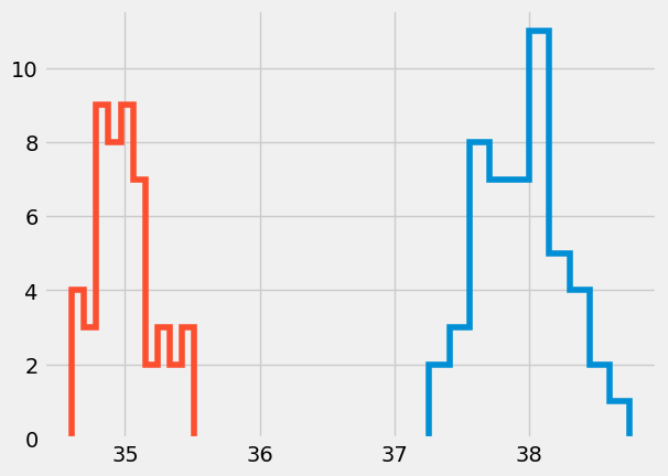
In the first, boxplot we see that for all sets of 100 throws Pat’s average work is higher than Jim’s average work. In the second histogram, we see the same information as the boxplot, but also the number of times the average was measured over the 50 trial sets. For example, the most likely average for Jim happened 9 times out of 50 at 35 J while Pat’s average happened 11 times just over 38 J.
T-test and the p-value for reporting significance#
This process is the same idea that William Gossett proposed in the formulation of the Student t-test. Rather than trying to prove that the two data sets are different, he built a test to see if the 2 means of the data sets were different assuming the mean is calculated from randomly sampled normally distributed data sets.
The T-test is now a standard way for scientists and engineers to discuss “how likely it is that any observed difference between groups is due to chance. Being a probability, P can take any value between 0 and 1” What does the P-value mean? Dahiru and Dip 2008. Let’s look at the p-value for 5 of the 50 data sets we made
from scipy.stats import ttest_ind
for i in range(0, 50, 10):
    print(ttest_ind(set_01[i, :], set_02[i,:]))
TtestResult(statistic=7.312243316551024, pvalue=6.360006381351198e-12, df=198.0)
TtestResult(statistic=7.287116791592907, pvalue=7.36799888979028e-12, df=198.0)
TtestResult(statistic=8.310616638454743, pvalue=1.4971760525056898e-14, df=198.0)
TtestResult(statistic=9.126645222590865, pvalue=8.222918423054348e-17, df=198.0)
TtestResult(statistic=10.319980173376308, pvalue=2.962493630516092e-20, df=198.0)
In all 5 data sets, the p-value is much less than 1%. The largest is 7.4e-12%. With 100 data points, and a standard deviation of equal to the difference between the means, we can be almost certain that the difference in the means is not by chance. Thus we reject this null hypothesis.
Pat is stronger than Jim
When is the p-value < 0.05?#
Now, lets decrease the number of times we measure Pat and Jim’s throwing work. We will only create 5 measurements of work from the normal distributions, but do the same experiment 50 times again.
set_01 = rng.normal(loc = 38, scale = 3, size = (50,5))
set_02 = rng.normal(loc = 35, scale = 2, size = (50, 5))

mean_01 = np.mean(set_01, axis = 1)
mean_02 = np.mean(set_02, axis = 1)

plt.boxplot([mean_01, mean_02], labels=['Pat avg', 'Jim Avg'])
plt.title('range of means using x50 sets of 5 data points\nlocated at 0 and 1')
Text(0.5, 1.0, 'range of means using x50 sets of 5 data points\nlocated at 0 and 1')
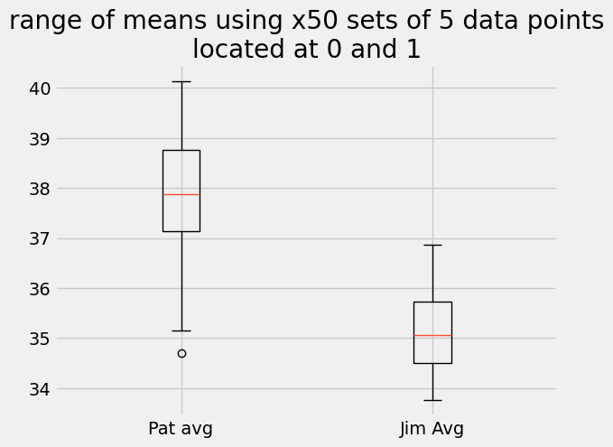
The population means are still where we expect them, at 68 and 65, but each set has a sample mean that varies from 65 to 71 and 63 to 67 for the \(\times 5\) data points.
for i in range(0, 50, 10):
    print(ttest_ind(set_01[i, :], set_02[i,:]))
TtestResult(statistic=1.152311308480025, pvalue=0.28246157139879224, df=8.0)
TtestResult(statistic=2.980630022687678, pvalue=0.017583498894211423, df=8.0)
TtestResult(statistic=1.7210662829147845, pvalue=0.12354561386016819, df=8.0)
TtestResult(statistic=-0.1759509471479071, pvalue=0.8647047810857478, df=8.0)
TtestResult(statistic=0.47500445800359664, pvalue=0.6474812142027704, df=8.0)
In the case of using 5 randomly sampled values from the normal distributions, the chance that the means are equal is as high as 86% and as low as 1.7%. This means we cannot claim the results are statistically significant even though we know that Pat’s set_01 has a mean of 68 J and Jim’s set_02 has a mean of 65 J.
The data does not support that Pat is stronger than Jim.
Why can’t we tell the difference between means now?#
This might seem strange that we built 2 random numbers with different means and sometimes we can tell the difference and other times we can’t. The main thing we changed in these two mini experiments with Pat and Jim was the number of measurements. Just like how we had a better estimate of \(\pi\) with more data points we get a better estimate of the means with more measurements.
So, if we have two measurements, Pat and Jim that seem the same we have two options:
shrug our shoulders and say
Pat == Jimkeep taking measurements until we can say
Pat > Jim
The very important point of using a statistical comparison is that it does not prove two random measurements are the same or different. We can only say that there is a chance that the sample measurements we made are from different random distributions.
Throwing distance#
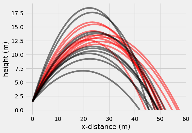
Enough of this talk of strength and work, let’s get Pat and Jim out in the field and start throwing some baseballs. How far can they throw the ball?
work is energy, so we can say W = kinetic energy
\(W = \frac{1}{2}mv^2\rightarrow v = \sqrt{\frac{2 W}{m}}\)
where a baseball is
and farthest distance thrown is \(\theta=45^o\pm5^o\)
so our distance, x, and height, y, are now:
\(x(t) = v\cos(\theta)t\)
\(y(t) = 1.5 + v\sin(\theta)t -\frac{g}{2}t^2\)
N_throws = 10
Pat_W = rng.normal(loc = 38, scale = 3, size = (N_throws,))
Jim_W = rng.normal(loc = 35, scale = 2, size = (N_throws,))

Pat_angle = rng.normal(loc = np.pi/4, scale = 5/180*np.pi, size = (N_throws,))
Jim_angle = rng.normal(loc = np.pi/4, scale = 5/180*np.pi, size = (N_throws,))

Pat_v = np.sqrt(2*Pat_W/0.15)
Jim_v = np.sqrt(2*Jim_W/0.15)

t_N = 50 # number of timesteps for path results
Pat_x = np.zeros((t_N, N_throws))
Pat_y = np.zeros((t_N, N_throws))
Jim_x = np.zeros((t_N, N_throws))
Jim_y = np.zeros((t_N, N_throws))
for i in range(N_throws):
    Pat_tmax = np.roots([-9.81/2, Pat_v[i]*np.sin(Pat_angle[i]), 1.5]).max()
    Jim_tmax = np.roots([-9.81/2, Jim_v[i]*np.sin(Jim_angle[i]), 1.5]).max()
    t = np.linspace(0, Pat_tmax, t_N)
    Pat_x[:,i] = Pat_v[i]*np.cos(Pat_angle[i])*t
    Pat_y[:,i] = 1.5 + Pat_v[i]*np.sin(Pat_angle[i])*t - 9.81*t**2/2

    t = np.linspace(0, Jim_tmax, t_N)
    Jim_x[:,i] = Jim_v[i]*np.cos(Jim_angle[i])*t
    Jim_y[:,i] = 1.5 + Jim_v[i]*np.sin(Jim_angle[i])*t - 9.81*t**2/2
plt.plot(Pat_x, Pat_y, 'r-', alpha = 0.5)
plt.plot(Jim_x, Jim_y, 'k-', alpha = 0.5)
plt.xlabel('x-distance (m)')
plt.ylabel('height (m)');
ttest_ind(Pat_x[-1, :], Jim_x[-1, :])
TtestResult(statistic=2.259841261689777, pvalue=0.03646659879452726, df=18.0)
plt.hist(Pat_x[-1, :],
histtype='step',
linewidth = 4,
label = 'Pat',
density = True,)
#bins = np.linspace(50,80, 31))
plt.hist(Jim_x[-1, :],
histtype = 'step',
linewidth = 4,
label = 'Jim',
density = True,)
plt.legend();
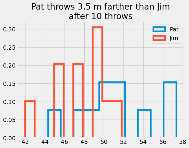
plt.title('Pat throws {:1.1f} m farther than Jim\nafter {} throws'.format(np.mean(Pat_x[-1, :]- Jim_x[-1, :]), N_throws))
Text(0.5, 1.0, 'Pat throws 3.5 m farther than Jim\nafter 10 throws')