Kinematic solutions for a piston-crank system

In this notebook, we begin creating the piston-crank kinematic constraints and solutions for positions, orientations, and speeds of the 4 parts:
ground support \([x^1,~y^1,~\theta^1]\)
crank arm \([x^2,~y^2,~\theta^2]\)
connector arm \([x^3,~y^3,~\theta^3]\)
piston \([x^4,~y^4,~\theta^4]\)
The constraints are such that,
$$C(q,~t) = 0$$
$$C(q,t) = \left[ \begin{array}{c} x^{1} - 0 \\ y^{1} - 0 \\ \theta^{1} - 0 \\ x^2 - \frac{L^2}{2}\cos\theta^{2} - x^{1} \\ y^2 - \frac{L^2}{2}\sin\theta^{2} - y^{1} \\ x^3 - \frac{L^3}{2}\cos\theta^{3} - x^2 - \frac{L^2}{2}\cos\theta^{2} \\ y^3 - \frac{L^3}{2}\sin\theta^{3} - y^2 - \frac{L^2}{2}\sin\theta^{2} \\ x^4 + 0 - x^3 - \frac{L^3}{2}\cos\theta^{3} \\ y^4 + 0 - y^3 - \frac{L^3}{2}\sin\theta^{3} \\ y^4 - 0 \\ \theta^4 - 0 \\ \theta^1 - \omega t - \theta_0 \end{array} \right]$$
using Symbolics, Plots, NonlinearSolve, ModelingToolkitusing ModelingToolkit: t_nounits as t, D_nounits as Dimport LatexifySet up variables for CAS
Here, we set up the simulation variables for the slider-crank system. The Computer Algebra System (CAS) allows us to compute exact derivatives and functions before we solve the numerical problems.
begin
    q = @variables x₁, y₁, θ₁, x₂, y₂, θ₂, x₃, y₃, θ₃, x₄, y₄, θ₄
    L2 = 0.15
    L3 = 0.35
    ω = 150 # rad/s
    θ₀ = 0 # rad initial angle
end
0
The CAS variable, C(q,t) plugs in the 12 degrees of freedom into the 12 constraint equations.
begin
    C(q,t) = [q[1] - 0;
             q[2] - 0;
             q[3] - 0;
             q[4] - L2/2*cos(q[6]) - q[1];
             q[5] - L2/2*sin(q[6]) - q[2];
             q[7] - L3/2*cos(q[9]) - q[4] - L2/2*cos(q[6]);
             q[8] - L3/2*sin(q[9]) - q[5] - L2/2*sin(q[6]);
             q[10] - q[7] - L3/2*cos(q[9]);
             q[11] - q[8] - L3/2*sin(q[9]);
             q[11] - 0;
             q[12] - 0;
             q[6] - ω*t - θ₀]
    C(q, t)
end
$$\begin{equation} \left[ \begin{array}{c} \mathtt{x{_1}} \\ \mathtt{y{_1}} \\ \mathtt{\theta{_1}} \\ - \mathtt{x{_1}} + \mathtt{x{_2}} - 0.075 ~ \cos\left( \mathtt{\theta{_2}} \right) \\ - \mathtt{y{_1}} + \mathtt{y{_2}} - 0.075 ~ \sin\left( \mathtt{\theta{_2}} \right) \\ - \mathtt{x{_2}} + \mathtt{x{_3}} - 0.175 ~ \cos\left( \mathtt{\theta{_3}} \right) - 0.075 ~ \cos\left( \mathtt{\theta{_2}} \right) \\ - \mathtt{y{_2}} + \mathtt{y{_3}} - 0.075 ~ \sin\left( \mathtt{\theta{_2}} \right) - 0.175 ~ \sin\left( \mathtt{\theta{_3}} \right) \\ - \mathtt{x{_3}} + \mathtt{x{_4}} - 0.175 ~ \cos\left( \mathtt{\theta{_3}} \right) \\ - \mathtt{y{_3}} + \mathtt{y{_4}} - 0.175 ~ \sin\left( \mathtt{\theta{_3}} \right) \\ \mathtt{y{_4}} \\ \mathtt{\theta{_4}} \\ - 150 ~ t + \mathtt{\theta{_2}} \\ \end{array} \right] \end{equation}$$
Then, computing Jacobians is a function call to find all of the partial derivatives in the 12x12 matrix.
dCdq(q, t) = Symbolics.jacobian(C(q, t), q)dCdq (generic function with 1 method)
dCdq(q, t)$$\begin{equation} \left[ \begin{array}{cccccccccccc} 1 & 0 & 0 & 0 & 0 & 0 & 0 & 0 & 0 & 0 & 0 & 0 \\ 0 & 1 & 0 & 0 & 0 & 0 & 0 & 0 & 0 & 0 & 0 & 0 \\ 0 & 0 & 1 & 0 & 0 & 0 & 0 & 0 & 0 & 0 & 0 & 0 \\ -1 & 0 & 0 & 1 & 0 & 0.075 ~ \sin\left( \mathtt{\theta{_2}} \right) & 0 & 0 & 0 & 0 & 0 & 0 \\ 0 & -1 & 0 & 0 & 1 & - 0.075 ~ \cos\left( \mathtt{\theta{_2}} \right) & 0 & 0 & 0 & 0 & 0 & 0 \\ 0 & 0 & 0 & -1 & 0 & 0.075 ~ \sin\left( \mathtt{\theta{_2}} \right) & 1 & 0 & 0.175 ~ \sin\left( \mathtt{\theta{_3}} \right) & 0 & 0 & 0 \\ 0 & 0 & 0 & 0 & -1 & - 0.075 ~ \cos\left( \mathtt{\theta{_2}} \right) & 0 & 1 & - 0.175 ~ \cos\left( \mathtt{\theta{_3}} \right) & 0 & 0 & 0 \\ 0 & 0 & 0 & 0 & 0 & 0 & -1 & 0 & 0.175 ~ \sin\left( \mathtt{\theta{_3}} \right) & 1 & 0 & 0 \\ 0 & 0 & 0 & 0 & 0 & 0 & 0 & -1 & - 0.175 ~ \cos\left( \mathtt{\theta{_3}} \right) & 0 & 1 & 0 \\ 0 & 0 & 0 & 0 & 0 & 0 & 0 & 0 & 0 & 0 & 1 & 0 \\ 0 & 0 & 0 & 0 & 0 & 0 & 0 & 0 & 0 & 0 & 0 & 1 \\ 0 & 0 & 0 & 0 & 0 & 1 & 0 & 0 & 0 & 0 & 0 & 0 \\ \end{array} \right] \end{equation}$$
ω150
begin
    N = 100
    tN = LinRange(0, 2*pi/ω, N)
    q_sol = zeros(length(tN), 12)
    dq_sol = zeros(length(tN), 12)

    partialCt = Symbolics.derivative.(C(q,t), t)

    local u0 = [0 0 0 L2/2 0 0 L2+L3/2 0 0 L2+L3 0 0]
    # 1. Define nonlinear equations from your constraint function
    eqs = 0 .~ C(q, t)

    # 2. Build and complete the nonlinear system
    @named constraint_system = NonlinearSystem(eqs, q, [t])
    constraint_system = complete(constraint_system)
    for (i, t0) in enumerate(tN)

        initial_guess = Dict(q[i] => u0[i] for i in range(1,12))

        problem = NonlinearProblem(
            constraint_system,
            merge(initial_guess,
            Dict(t => t0))
        )

        solution = solve(problem)
        u0 = solution.u

        q_sol[i,:] = solution.u

        sol_dict = Dict(q[j] => q_sol[i, j] for j in range(1, 12))
        lhs = Symbolics.substitute(dCdq(q, t0), sol_dict, fold=Val(true))
        rhs = Symbolics.substitute(-partialCt, sol_dict, fold=Val(true))
        solv = Symbolics.value.(lhs\rhs)
        dq_sol[i,:] .= solv
    end
end
q_sol[1, 1:3:end]4-element Vector{Float64}:
0.0
0.075
0.32499999999999996
0.5
begin


    @gif for i in range(1, length(tN))
        scatter(q_sol[:,1], q_sol[:,2], m = :circle, label = "ground support")
        plot!(q_sol[:,4], q_sol[:,5], label = "crank arm")
        plot!(q_sol[:,7], q_sol[:,8], label = "connector arm")
        plot!(q_sol[:,10], q_sol[:,11], label = "piston")

        plot_rectangle(q_sol[i, 1:3], [0.02, 0.02], label = "")
        plot_rectangle(q_sol[i, 4:6], [L2, 0.01], label = "")
        plot_rectangle(q_sol[i, 7:9], [L3, 0.01], label = "")
        plot_rectangle(q_sol[i, 10:12], [0.01, 0.05], label = "")
        plot!(aspect_ratio = 1,
              xlims = [2*minimum(q_sol[:, 1:3:end]),
                       2*maximum(q_sol[:, 1:3:end])],
             ylims = [4*minimum(q_sol[:, 2:3:end]),
                       4*maximum(q_sol[:, 2:3:end])])

    end

end
begin
    p = plot(title = "speeds of parts")
    for i in range(1, 12, step = 1)
        plot!(p, tN,
              dq_sol[:, i],
              label = q[i],
             linewidth = 3)
    end
p
end
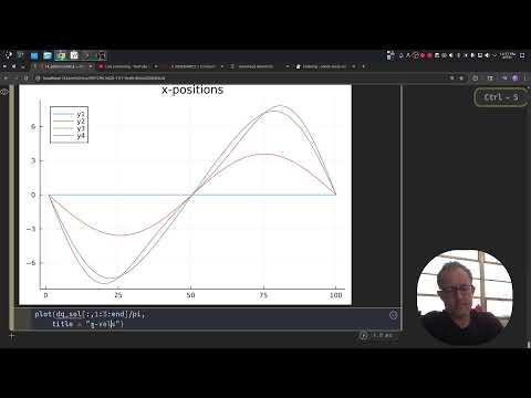
plot(180*dq_sol[:,3:3:end]/pi,
    title = "rotation rates")
Wrapping up
In this notebook, we built 12 kinematic constraints on 4 moving parts with a total of \(4\times 3 = 12~DOFs\). The result is a complete kinematic set of constraints with zero degrees of freedom.
In order to solve for the geometry and motion of these parts, we took three steps:
solve the constraint equations for \(\mathbf{q}\rightarrow C(\mathbf{q},t)=\mathbf{0}\)
solve for the velocities using \(\mathbf{q}\) at time, t, \(\frac{\partial C}{\partial \mathbf{q}} = -C_t\dot{\mathbf{q}}\)
visualize and check results with plots and tables (even cool animations)
Built with Julia 1.12.5 and
Latexify 0.16.10ModelingToolkit 11.10.0
NonlinearSolve 4.16.0
Plots 1.41.6
Symbolics 7.17.0
To run this tutorial locally, download this file and open it with Pluto.jl.