import numpy as np
from scipy.stats import norm, t

import matplotlib.pyplot as plt
import pandas as pd
plt.rcParams.update({'font.size': 22})
plt.rcParams['lines.linewidth'] = 3

import check_lab02 as p
Note: If you download this notebook to edit offline in the computer lab, you will need this file (right click -> save as) in the same directory as the .ipynb file
ME 3263 - Laboratory #2
What is a Strain Gauge?
A strain gauge consists of a looped wire that is embedded in a thin backing. Two copper coated tabs serve as solder points for the leads. See Figure 1a. The strain gauge is mounted to the structure, whose deformation is to be measured. As the structure deforms, the wire stretches (increasing its net length ) and its electrical resistance changes: \(R=\rho L/A\), where \(\rho\) is the material resistivity, \(L\) is the total length of the wire, and \(A\) is the cross sectional area of the wire. Note that as \(L\) increases, the cross sectional area changes as well due to the Poisson contraction; the resistivity also changes.
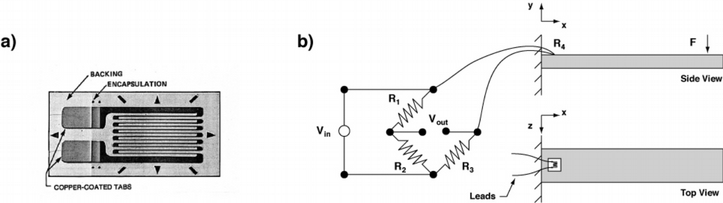
Figure 1: a) A typical strain gauge. b) One common setup: the gauge is mounted to measure the x-direction strain on the top surface. It’s engaged in a quarter bridge configuration of the Wheatstone bridge circuit.
Validating static strain gauge measurements
In this lab we will calibrate strain measurements using Euler-Bernouli beam theory kinematics [1]. The axial strain in a beam is directly proportional to the distance from the neutral axis and curvature:
\(\epsilon_x=-\kappa z\). (1)
Where \(\epsilon_x\) is the strain in the material, \(z\) is the distance from the neutral axis, and \(\kappa\) is the curvature of the beam. \(\kappa\) is approximated as the second derivative of the displacement of the center axis:
\(\kappa=\frac{d^2 w}{dx^2}\). (2)
Equations 1 and 2 relate beam deflection to axial strain. These are called kinematic equations because they define the geometry of the beam deflection.
The Euler-Bernouli beam theory uses Newton’s second law (kinetics) and Hooke’s law (constitutive) to derive the linear equations of motion for one dimensional deformable objects [1,4]. The relation between a static applied force \(q(x)\) and static deflection \(w(x)\) is:
\(\frac{\partial^2}{\partial x^2}\left(EI\frac{\partial^2 w}{\partial x^2}\right)=q(x)\) (3)
where \(E\) is the Young’s modulus, \(x\) is the distance along the neutral axis, and \(I\) is the second moment of area of the beam’s cross-section. For a rectangular cross-section \(b \times t\), width by thickness the second moment of area is:
\(I=\frac{bt^3}{12}\). (4)
We can design our strain gage validation such that \(E\) and \(I\) are not necessary. A cantilevered (clamped) beam of length \(L\) that is deflected by a distance \(\delta\) at the free end has the following boundary conditions for its static deflection:
\(w(0)=0\), \(w'(0)=0\), \(w(L)=\delta\), and \(w''(L)=0\)
Therefore, the functions \(w(x)\) and \(w''(x)\) can be determined by integrating equation 3 four times and using the four boundary conditions:
\(w(x)=-\frac{1}{2}\left(\frac{\delta}{L^3}x^3-3\frac{\delta}{L^2}x^2\right)\) (5a)
and the curvature
\(w''(x)=-\left(3\frac{\delta}{L^3}x-3\frac{\delta}{L^2}\right)\) (5b)
Using equations 1,2, and 5, the only quantities needed to determine strain at a given location on a linear, homogeneous beam are \(z\), \(\delta\), and \(L\).
Below are two functions that calculate displacement and curvature given a cantilevered beam of length L that is deflected by a distance delta at its free end.
def disp_at_x(x,L,delta):
    '''returns the displacement w(x) given the position, x,
    length of bar, L, and displacement at L, delta'''
    wx=-1/2*(delta/L**3*x**3-3*delta/L**2*x**2)
    return wx

def k_at_x(x,L,delta):
    '''returns the curvature w''(x) given the position, x,
    length of bar, L, and displacement at L, delta'''
    wx=-(3*delta/L**3*x-3*delta/L**2)
    return wx
w20mm=disp_at_x(20,400,10)
k20mm=k_at_x(20,400,10)
print('displacement of 400 mm bar deflected 10 mm, 20 mm from support =%1.3f mm'%w20mm)
print('   curvature of 400 mm bar deflected 10 mm, 20 mm from support =%1.3f 1/m'%(k20mm*1000))
displacement of 400 mm bar deflected 10 mm, 20 mm from support =0.037 mm
   curvature of 400 mm bar deflected 10 mm, 20 mm from support =0.178 1/m
Example Problem 1
If your beam is 400 mm long by 10 mm thick and it deflects 15 mm at the tip, determine the following:
a. displacement of the beam 20 mm from the base. Save as w20
b. the curvature of the beam 20 mm from the base. Save as k20
c. the strain of the beam 20 mm from the base. Save as e20
# your work here

p.check_p01(w20,k20,e20)
---------------------------------------------------------------------------
NameError                                 Traceback (most recent call last)
/tmp/ipykernel_1712/232341384.py in <module>
      1 # your work here
      2
----> 3 p.check_p01(w20,k20,e20)

NameError: name 'w20' is not defined
Visualizing deflection and curvature
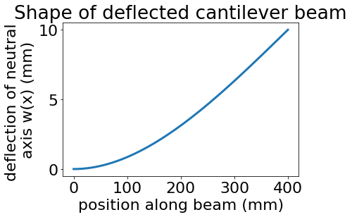
We can use the above expressions for \(w\) and \(w''\) to plot the deflection and curvature of a cantilevered beam:
x=np.linspace(0,400)
wx=disp_at_x(x,400,10)
plt.plot(x,wx)
plt.xlabel('position along beam (mm)')
plt.ylabel('deflection of neutral \naxis w(x) (mm)')
plt.title('Shape of deflected cantilever beam')
Text(0.5, 1.0, 'Shape of deflected cantilever beam')
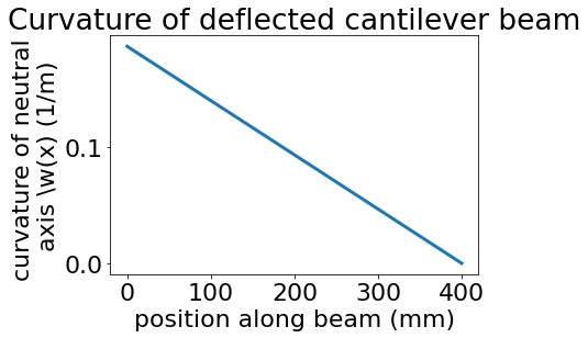
x=np.linspace(0,400)
kx=k_at_x(x,400,10)
plt.plot(x,kx*1000)
plt.xlabel('position along beam (mm)')
plt.ylabel('curvature of neutral \naxis \\w(x) (1/m)')
plt.title('Curvature of deflected cantilever beam')
Text(0.5, 1.0, 'Curvature of deflected cantilever beam')
Example Problem 2
If your beam is 400 mm long by 10 mm thick and it deflects 15 mm at the tip, determine the position along the beam for the following:
a. Where is the maximum deflection in the beam? save as x_max_defl
b. Where is the maximum curvature in the beam? save as x_max_curv
c. Where is the maximum strain in the beam? save as x_max_strain
#your work here

p.check_p02(x_max_defl,x_max_curv,x_max_strain)
---------------------------------------------------------------------------
NameError                                 Traceback (most recent call last)
<ipython-input-3-ec3929850900> in <module>
      1 #your work here
      2
----> 3 p.check_p02(x_max_defl,x_max_curv,x_max_strain)

NameError: name 'x_max_defl' is not defined
Task 1: Validate Strain Gauge Measurements
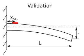
Figure 2: Diagram of the validation process. The strain gauge is placed at a distance \(x_{SG}\) from the cantilever support. A linear-elastic beam of length \(L\) is deflected by distance, \(\delta\).
Apply a known tip displacement as seen in Figure 2.
Measure and record the strain at your strain gage location, the displacement, \(\delta\), and position where load was applied, \(L\).
Calculate the strain at the location of the strain gage using equations 1,2, and 5a-b.
Compare the calculated and measured strain values
Measuring constitutive properties
Constitutive Model
Now that the strain gauge has been calibrated, we can use it to determine constitutive properties of our workpiece. Using measurements of strain, we wish to determine the Young’s modulus of the beam, \(E\). This measurement requires three components: kinematic (the geometric equations solved in the validation), kinetic (\(\sum{F}=0\)), and a constitutive model (Hooke’s Law). The constitutive equation for a linear-elastic beam subject to an applied moment is:
\(M=EI\kappa\). (6)
where \(M\) is the applied moment, \(E\) is the Young’s modulus, \(I\) is the second moment of inertia of the area of the beam, and \(\kappa\) is the curvature of the beam. The constant \(I\) is based upon the geometry from equation 4 (\(I=\frac{bt^3}{12}\)). The material constant \(E\) is unknown.
Task 2: Collect Data for a Constitutive Model
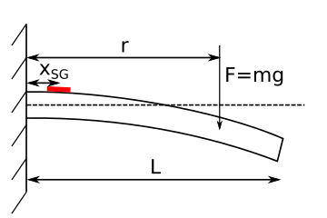
Figure 3: A linear-elastic beam of length \(L\) has a force applied at distance, \(r\). The strain gauge is placed at a distance \(x\) from the cantilever support.
Measure and record the length, width, and thickness of your beam for use in calculating the second moment of area. Remember that your ruler can only record to the millimeter, and your calipers to the hundredth of a millimeter.
There are notches cut into your beam. Use them to attach varying weights to apply forces at varying distances, \(r\), from the support (as seen in Figure 3). Increasing the weight or the distance at which the weight is applied will increase the applied moment.
Record the trial no., strain, force, distance, and moment for each combination of weight and distance. Use at least two trials per measurement.
Fitting your data to your model
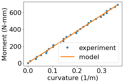
Once you have collected a number of data points for \(\kappa\) and \(M\), you can use a linear regression to determine the slope of the data. The constitutive model in equation (6) predicts that the moment and curvature will be related by a proportional constant, \(EI\). If we know \(EI\), the total squared error is as such
\(SSE=\sum_i^N{(M_i-EI\kappa_i)^2}\) (7)
where SSE is the sum of squares error between the predicted moment and measured moment for the \(i^{th}\) measurement with \(N\) total measurements [2]. We can choose a of \(EI\) that minimizes \(SSE\), but it will never be zero. Below is an example calculation for a linear least squares regression in python for a beam with cross-section \(12\times3\) mm.
k=np.array([6.95685737e-07, 9.93992373e-06, 3.25200211e-05, 3.55750721e-05,
       5.32023782e-05, 7.48128585e-05, 7.61625461e-05, 8.54476229e-05,
       1.02089509e-04, 1.02841452e-04, 1.32351731e-04, 1.43996022e-04,
       1.45204793e-04, 1.56867759e-04, 1.73435915e-04, 1.95625232e-04,
       2.00670618e-04, 2.12900332e-04, 2.24582886e-04, 2.41141396e-04,
       2.45991618e-04, 2.55608426e-04, 2.76117673e-04, 2.96128593e-04,
       3.07157389e-04, 3.20509718e-04, 3.20363196e-04, 3.35535814e-04,
       3.53706984e-04, 3.64130433e-04])
M=np.array([ 0.        ,  23.82866379,  47.65732759,  71.48599138,
        95.31465517, 119.14331897, 142.97198276, 166.80064655,
       190.62931034, 214.45797414, 238.28663793, 262.11530172,
       285.94396552, 309.77262931, 333.6012931 , 357.4299569 ,
       381.25862069, 405.08728448, 428.91594828, 452.74461207,
       476.57327586, 500.40193966, 524.23060345, 548.05926724,
       571.88793103, 595.71659483, 619.54525862, 643.37392241,
       667.20258621, 691.03125   ])
from scipy.optimize import curve_fit

def func(x,EI):
    return EI*x

EI,pcov=curve_fit(func, k, M)
EI_error=np.sqrt(pcov[0,0])
I=12*3**3/12.0
print("Best fit for Young's Modulus is %1.1f +/- %1.1f GPa"%(EI/I*1e-3,EI_error/I*1e-3))

plt.plot(k*1e3,M,'o',label='experiment')
plt.plot(k*1e3,func(k,EI),label='model')
plt.legend()
plt.xlabel('curvature (1/m)')
plt.ylabel('Moment (N-mm)')
Best fit for Young's Modulus is 70.2 +/- 0.3 GPa
Text(0, 0.5, 'Moment (N-mm)')
Note:
The least-squares method used above can be used to fit any function to a data set. You would just need to update the func definition to return the desired function based upon your unkown fitting constants.
The outout popt is the covariance matrix [3]. In practice, we can use the square root of the diagonal terms to estimate the error in our least-squares fit. We make a few assumptions when performing this best-fit:
There is a random error in the measured dependent variable (here the moment \(M\)).
There is no error in the reported independent variable (here the curvature \(\kappa\)).
The measured dependent variables are uncorrelated with the measured error
The random error has a mean of zero
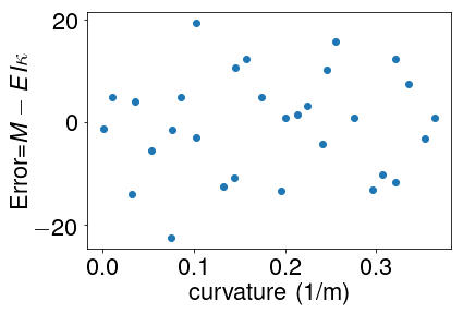
We can test assumption 4 by plotting the “residuals” of the fit i.e. the error. The plot below demonstrates that our data has a mean error of 0 and is uncorrelated with the random error.
Our best-fit model has removed systematic uncertainty, but it cannot account for random uncertainty.
plt.plot(k*1e3,M-func(k,EI),'o')
plt.xlabel('curvature (1/m)')
plt.ylabel(r'Error=$M-EI\kappa$')
Text(0,0.5,'Error=$M-EI\\kappa$')
Task 3: Determine Young’s Modulus
Using a linear least squares regression, determine the Young’s modulus, \(E\), of your beam
Propagation of Error
If the physical quantities involved in the calculation (e.g., the thickness of the beam) are not measured properly, you can have large systematic errors in your results.
Example Problem 3
In the example E calculation above, the width of the beam was 12 mm and the thickness of the beam was 3 mm. On the line,
I = 12*3**3/12.0
Change the thickness to 3.1 mm and calculate \(E\). Save the value as E31
# Your work here

p.check_p03(E31)
---------------------------------------------------------------------------
NameError                                 Traceback (most recent call last)
<ipython-input-4-1e6b442bf583> in <module>
      1 # Your work here
      2
----> 3 p.check_p03(E31)

NameError: name 'E31' is not defined
Task 4: Determine the uncertainty in your estimate of Young’s modulus
Each measurement you have taken over the course of this lab has its own associated uncertainty, and that uncertainty propagates through any calculated quantities. Your calculations of moment of inertia from geometry of the beam: \(I=\frac{bt^3}{12}\), curvature from strain: \(\kappa=-\frac{\epsilon}{z}\), and moment from applied mass: \(M=rF\) all possess uncertainties due to the measured quantities involved in their calculation.
Using the method we learned in class for calculating propagation of error, determine the uncertainties in \(I\), \(\kappa\), and \(M\). With these uncertainties, calculate the uncertainty in \(E\) obtained by the expression \(E=\frac{M}{I\kappa}\).
Alternatively, substitute the experssions for \(I\), \(\kappa\), and \(M\) in to \(E=\frac{M}{I\kappa}\), then take the partial derivatives of \(E=f(b,t,r,\epsilon\)) to find the overall sensitivity to each variable.
To estimate the overall uncertainty in the experiment, it is acceptable to use the means of all measured values in the calculation - the mean of \(r\), the mean of \(\epsilon\), etc.
The uncertainties in your measurements of length can be assumed to be zero-order. In other words, consider only the errors due to instrument resolution: \(u_{xi}=\frac{resolution}{2}\).
The uncertainty in your strain measurements can be estimated in two ways for this lab. They will give different results, but both will work for our purposes. First, you may record the “drift” value of your strain gauge after all measurements have been taken. This is the readout of the strain gauge in Lab View when the beam is under no applied moment. Second, you may use the difference between calculated and measured strain from your calibration in Task 1.
Assume the applied mass is known perfectly - i.e., there is no uncertainty to the force applied to the beam.
Your Report
Describe and discuss the results you obtained for the measurement of \(E\).
Follow the established format for lab reports: Introduction, Methods, Results & Discussion, Conclusion
References
References
Sutton, M. A., Orteu, J. J., & Schreier, H. (2009). Image correlation for shape, motion and deformation measurements: basic concepts, theory and applications. Springer Science & Business Media.
F.P. Beer and E.R. Johnson, Mechanics of Materials, 2nd Edition, McGraw-Hill, 1992.
S. Chapra, Numerical Methods for Engineers, ch. 14-15, 6th Edition, McGraw-Hill, 2009.
C. Salter, Error Analysis Using the Variance–Covariance Matrix, J. of Chem. Ed., 2000.