animate_lines - create NumPy array animations

The module creates matplotlib animations from 2D and 3D NumPy arrays

---

source

default_fig_setup

 default_fig_setup ()

A boiler-plate wrapper to get a clean figure and axis from animations

/opt/hostedtoolcache/Python/3.9.16/x64/lib/python3.9/site-packages/fastcore/docscrape.py:225: UserWarning: potentially wrong underline length... 
Parameters: 
---------- in 
`animate_lines(X, Y)` is a function that takes x2 3D arrays, `X` and `Y` 
and returns an animation of the changing lines...
  else: warn(msg)
/opt/hostedtoolcache/Python/3.9.16/x64/lib/python3.9/site-packages/fastcore/docscrape.py:225: UserWarning: Unknown section Returns:
  else: warn(msg)

---

source

animate_lines

 animate_lines (X, Y, xlabel='x-position', ylabel='y-position',
                setup_fig_function=<function default_fig_setup>, xlims=[],
                ylims=[], labels=[], linewidth=5, legend=False,
                interval:int=200, **plotargs)

animate_lines(X, Y) is a function that takes x2 3D arrays, X and Y and returns an animation of the changing lines

The X and Y arrays need to be arranged in 3D arrays such that,

X[line_N, point_i, time_j], Y[line_N, point_i, time_j]

where each line is arranged in columns and the next frame is aranged in the third dimension of the array

If you are plotting a single line, you can use the columns as the timestep e.g. 

X[point_i, time_j], Y[point_i, time_j]

the function will add an extra axis to the beginning of the arrays as such

X[:, np.new_axis :], Y[:, np.new_axis, :]

Parameters:

X: The x-axis data for the animated lines, its shape is such that each column is a set of x-values for a given line and each frame is organized along the third dimension Y: The y-axis data for the animated lines, its shape is such that each column is a set of y-values for a given line and each frame is organized along the third dimension xlabel: plot x-axis label, default is ‘x-position’, ylabel: plot y-axis label, default is ‘y-position’, setup_fig_function: a function that returns fig and ax that can be used to plot static lines before animating, default is an empty plot xlims: Manually set the x-axis limits. If its not specified, the animation uses 1.1*(max&min) ylims: [], labels: [], linewidth: 5 legend: False, interval : int, default: 200 Delay between frames in milliseconds. plotargs: used as kwargs for matplotlib’s plot command

Set up X and Y variables that are functions of time

each column is a single line, \(x-\) or \(y-\) values. Here, the first point in time is called with all columns and all rows. Each \((x_{zN},~y_{zN})\) is plotted as a single line for that animation frame. - lines that will be drawn are labeled \(a,~b,~...~z\), for 4 lines, there are 4 columns. - \(x-y\) coordinates are numbered \(1,~2,~...~N\), for 100 coordinates, there are 100 rows.

\(X[:,~ :,~ 0] = \left[\begin{array} ~x_{a1}(0) & x_{b1}(0) & ... & x_{z1}(0)\\ x_{a2}(0) & x_{b2}(0) & ... & x_{z2}(0)\\ x_{a3}(0) & x_{b2}(0) & ... & x_{z3}(0)\\ ... & ... & ... & ...\\ x_{aN}(0) & x_{bN}(0) & ... & x_{zN}(0) \end{array}\right]\)

\(Y[:,~ :,~ 0] = \left[\begin{array} ~y_{a1}(0) & y_{b1}(0) & ... & y_{z1}(0)\\ y_{a2}(0) & y_{b2}(0) & ... & y_{z2}(0)\\ y_{a3}(0) & y_{b2}(0) & ... & y_{z3}(0)\\ ... & ... & ... & ...\\ y_{aN}(0) & y_{bN}(0) & ... & y_{zN}(0) \end{array}\right]\)

The next time step would be,

\(X[:,~ :,~ 1] = \left[\begin{array} ~x_{a1}(\Delta t) & x_{b1}(\Delta t) & ... & x_{z1}(\Delta t)\\ x_{a2}(\Delta t) & x_{b2}(\Delta t) & ... & x_{z2}(\Delta t)\\ x_{a3}(\Delta t) & x_{b2}(\Delta t) & ... & x_{z3}(\Delta t)\\ ... & ... & ... & ...\\ x_{aN}(\Delta t) & x_{bN}(\Delta t) & ... & x_{zN}(\Delta t) \end{array}\right]\)

\(Y[:,~ :,~ 1] = \left[\begin{array} ~y_{a1}(\Delta t) & y_{b1}(\Delta t) & ... & y_{z1}(\Delta t)\\ y_{a2}(\Delta t) & y_{b2}(\Delta t) & ... & y_{z2}(\Delta t)\\ y_{a3}(\Delta t) & y_{b2}(\Delta t) & ... & y_{z3}(\Delta t)\\ ... & ... & ... & ...\\ y_{aN}(\Delta t) & y_{bN}(\Delta t) & ... & y_{zN}(\Delta t) \end{array}\right]\)

In this example, we create 4 vibration modes that vibrate while the amplitude decays,

\(y(t,~x) = A(t)\sin(\lambda x)\)

where - \(t\) time goes from 0-5 seconds with 50 steps - \(x\) is the x-axis variable that goes from 0 to \(2\pi\) units - \(A(t) = e^{-t/2}\cos(6t)\) is the oscillating and decaying amplitude - \(\lambda = \frac{1}{2},~1,~\frac{3}{2},~2\) are the wave shapes for 1/2-, full, 1.5 and 2x sine waves along the x-axis

t = np.linspace(0, 5)
x = np.linspace(0, 2*np.pi, 100)

y1 = np.sin(x/2)
y2 = np.sin(x)
y3 = np.sin(1.5*x)
y4 = np.sin(2*x)

A = np.exp(-t/2)*np.cos(6*t)

y = np.array([y1, y2, y3, y4]).T

Now, I set up the full 3D arrays for X and Y.

X.shape \(=(100, 4, 50) = (rows,~columns,~layers)\) - axis 0: each row is a constant \(x\)-value - axis 1: each column is a new line that will be drawn - axis 2: each layer is a new time step

X = np.zeros((len(x), y.shape[1], len(t)))
Y = np.zeros((len(x), y.shape[1], len(t)))

for i in range(len(t)):
    Y[:, :, i] = A[i]*y
    X[:, :, i] = np.array([x for i in range(y.shape[1])]).T

Observing a static image, the 1/2-sine wave is shown every \(5^{th}\) timestep.

for i in range(0, len(t), 5):
    plt.plot(X[:, 0, i], Y[:, 0, i])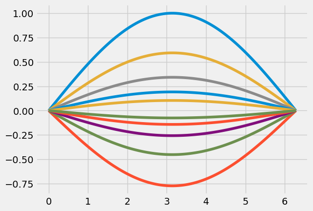

Now, I can plot the \(\times 4\) lines oscillating and watch the amplitudes decrease using the default parameters in

anim = animate_lines(X, Y, interval=84)

HTML(anim.to_html5_video())

I can also view the animation using Javascript HTML, which adds extra functionality to the video player,

HTML(anim.to_jshtml())

Once Loop Reflect