Solving Kinematic Constraints
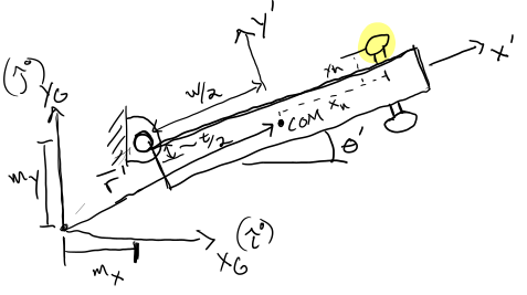
Moving door and the reference frames to define its motion in body-fixed and global coordinates.
Door Example Setup
A door is modeled as a rigid body with center of mass at \(R_1\) and rotation \(\theta_1\). A point such as the handle is located using offsets \((x_H, y_H)\): \(R_H = R_1 + x_H\,\mathbf{i}_1 + y_H\,\mathbf{j}_1\)
The hinge point, offset by door width \(W\) and thickness \(T\): \(R_{hinge}^{(1)} = R_1 - \frac{W}{2}\mathbf{i}_1 + \frac{T}{2}\mathbf{j}_1\)
The same hinge point expressed in ground coordinates: \(R_{hinge}^{(0)} = R_0 + M_x\mathbf{i}_0 + M_y\mathbf{j}_0\)
We use these hinge constraints to build \(\mathbf{C}(\mathbf{q},~t)\)
using NonlinearSolve,Plots, LatexifyTime‑Varying Constraint
If the door is pushed upward at constant speed: \(R_{1y} = 2t \quad \Rightarrow \quad \dot{R}_{1y} = 2\) This creates a third constraint to be incorporated into the system
begin
    #q = [x_1, y_1, θ_1]
    W = 1
    T = 3e-2
    mx = 0.0
    my = T/2
    C(q, p) = [q[1] - W/2*cos(q[3]) - T/2*sin(q[3]) - mx,
               q[2] - W/2*sin(q[3]) + T/2*cos(q[3]) - my,
               q[2] - 2*p - T/2]

end
C (generic function with 1 method)
begin
    time = LinRange(0, 0.25, 51)
    q_all = zeros(length(time), 3)
    for i in range(1, length(time))

        prob = NonlinearProblem(C, [0, 0, 0], time[i])
        sol = solve(prob)
        q_all[i, :] = sol
    end
end
plot(time, q_all)
C(q_all[51, :], time[51])3-element Vector{Float64}:
5.204170427930421e-18
6.609296443471635e-16
1.3877787807814457e-17
Solving the System speeds
At each timestep:
Position solve: find \(q\) such that \(C(q,t)=0\)
Velocity solve: solve linear system \(C_q \dot{q} = -C_t\)
begin
    dCdq(q, p) = [1 0 W/2*sin(q[3])-T/2*cos(q[3]);
              0 1 -W/2*cos(q[3])-T/2*sin(q[3]);
             0 1 0]
    Ct(q, p) = [0,0,2.0]
    dq_all = zeros(length(time), 3)
    for i in range(1, length(time))
        qt = q_all[i, :]
        sol = dCdq(qt, time[i])\Ct(qt, time[i])
        dq_all[i, :] = sol
    end
end
plot(time, dq_all)
plot_oriented_rectangle! (generic function with 1 method)
Animate the door motion
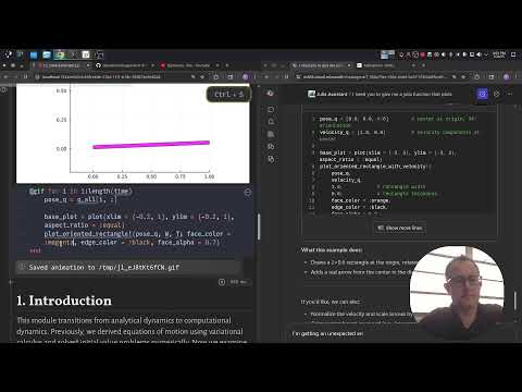
In this next step, we use plot_oriented_rectangle to show the door in a given position and orientation. The input to the Julia Assistant in copilot was,
"I need you to give me a julia function that plots a rectangle given its x,y position and orientation, theta in a vector q=[x, y, theta] and let me define its width and thickness for the plot"
Then, we use the @gif loop to watch the door open over time.
@gif for i in 1:length(time)
    pose_q = q_all[i, :]

    base_plot = plot(xlim = (-0.2, 1.5), ylim = (-0.5, 1), aspect_ratio = :equal)
    plot_oriented_rectangle!(pose_q, W, T; face_color = :magenta, edge_color = :black, face_alpha = 0.7)
end
Built with Julia 1.12.4 and
Latexify 0.16.10NonlinearSolve 4.16.0
Plots 1.41.6
To run this tutorial locally, download this file and open it with Pluto.jl.