Creating Kinematic Constraints

1. Introduction

This module transitions from analytical dynamics to computational dynamics. Previously, we derived equations of motion using variational calculus and solved initial value problems numerically. Now we examine how computers represent rigid-body systems through coordinates, constraints, and kinematics.

2. Multi‑Body Kinematics Overview

Computational dynamics focuses on rigid-body motion described through generalized coordinates. For a body:

• Position: \(R_1 = [x_1, y_1]^T\)

• Orientation: \(\theta_1\)

• Body-fixed axes: \(\mathbf{i}_1, \mathbf{j}_1\)

Any point on the body can be written: \(R = R_1 + x\,\mathbf{i}_1 + y\,\mathbf{j}_1\)

3. Door Example Setup

A door is modeled as a rigid body with center of mass at \(R_1\) and rotation \(\theta_1\). A point such as the handle is located using offsets \((x_H, y_H)\): \(R_H = R_1 + x_H\,\mathbf{i}_1 + y_H\,\mathbf{j}_1\)

The hinge point, offset by door width \(W\) and thickness \(T\): \(R_{hinge}^{(1)} = R_1 - \frac{W}{2}\mathbf{i}_1 + \frac{T}{2}\mathbf{j}_1\)

The same hinge point expressed in ground coordinates: \(R_{hinge}^{(0)} = R_0 + M_x\mathbf{i}_0 + M_y\mathbf{j}_0\)

Setting these equal produces constraint equations.

4. Rotation Matrix

To relate body-fixed and ground-fixed frames: \(A(\theta_1) = \begin{bmatrix} \cos\theta_1 & -\sin\theta_1 \\ \sin\theta_1 & \cos\theta_1 \end{bmatrix}\)

Thus: \(\mathbf{i}_1 = A(\theta_1)\mathbf{i}_0, \qquad \mathbf{j}_1 = A(\theta_1)\mathbf{j}_0\)

The transpose equals the inverse: \(A^{-1}(\theta_1) = A^T(\theta_1)\)

5. Constraint Equations

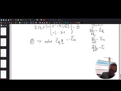
The hinge must satisfy: \(C(q) = R_1 + A(\theta_1) r_{hinge}^{(1)} - R_{hinge}^{(0)} = 0\) This expands into two scalar equations (x and y constraints).

6. Velocity Constraints

Taking the time derivative: \(\frac{d}{dt}C(q,t) = 0\) Applying the chain rule: \(C_q \, \dot{q} = -C_t\) where \(q = [x_1, y_1,\theta_1]^T\).

Differentiating the rotation matrix term yields: \(\frac{d}{dt}A(\theta_1) = A(\theta_1)\begin{bmatrix}0 & -\dot{\theta}_1 \ \dot{\theta}_1 & 0\end{bmatrix}\)

7. Adding a Time‑Varying Constraint

If the door is pushed upward at constant speed: \(R_{1y} = 2t \quad \Rightarrow \quad \dot{R}_{1y} = 2\) This creates a third constraint to be incorporated into the system.

8. Solving the System

At each timestep:

1. Position solve: find \(q\) such that \(C(q,t)=0\)

2. Velocity solve: solve linear system \(C_q \dot{q} = -C_t\)

These yield consistent positions and velocities that satisfy all kinematic constraints.

Wrapping Up

This framework provides:

• Rigorous description of rigid‑body motion

• Consistent enforcement of physical constraints

• Linear velocity equations even for nonlinear positions

• A foundation for forming differential‑algebraic equations used in multi‑body simulation

Computational dynamics transforms geometry, motion, and constraint information into forms solvable by numerical tools such as Julia, MATLAB, or Python.