Solving the damped pendulum equations of motion

The equations of motion for this damped oscillating system are as follows,

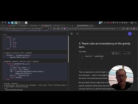
$$m\ddot{x} + \frac{mL}{2}\ddot{\theta}\cos\theta - \frac{mL}{2}\dot{\theta}^2\sin\theta + b\dot{x} + kx = 0$$
$$\frac{mL}{2}\ddot{x}\cos\theta + \frac{mL^2}{3}\ddot{\theta} + \frac{mgL}{2}\sin\theta = 0$$

using ModelingToolkit, OrdinaryDiffEq, Plots, Latexify

In order to solve for the motion of the pendulum, we assign values to the spring stiffness, damper, gravity, mass, and length of the compound pendulum system.

begin
    k = 2 # N/m
    b = 5 # kg/s
    g = 9.81 # m/s/s
    m = 0.1 # kg mass of pendulum bar
    L = 0.9 # m length of pendulum bar
end

0.9

Coupled equations of motion

In general, the motion of one degree of freedom can affect other degrees of freedom. This creates coupled differential equations. Each integration step requires a solution to the set of equations to find the acceleration of the degrees of freedom.

In this case, we create 2 functions:

a mass-matrix function, M(theta) that changes with angle
a pendulum! function that updates the changes in our 'state' variable derivatives, dy$=[\dot{x},~\dot{\theta},~\ddot{x},~\ddot{\theta}]$

of note for the pendulum! function is that the ! is a Julia convention that the first argument is being mutated
variable mutation is subtly different than "assigning" a value.
why mutate vs assign??: There are pros/cons to each. Here it makes sense since the value of dy is used, but not saved anywhere so its better to update with current values.

M(theta) = [m m*L/2*cos(theta);
    m*L/2*cos(theta) m*L^2/3]

M (generic function with 1 method)

function pendulum!(dy, y, params, time)
    # physical parameters 
    b, k, m, L, g = params

    x, theta, dx, dtheta = y
    
    dy[1:2] .= [dx, dtheta]
    
    rhs = [-b*dx-k*x+m*L*dtheta^2*sin(theta);
          -m*g*L/2*sin(theta)]

    dy[3:4] .= M(theta)\rhs
    return nothing
end

pendulum! (generic function with 1 method)

Compare damping terms and response

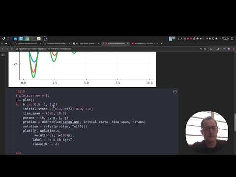
Here, we try 4 different damping terms to see what effect it has on the motion of the pendulum. Counterintuitively, the $b=1000~kg/s$ has the smallest effect on pendulum motion.

begin
# plots_array = []
P = plot()
for b in [0.5, 1, 1.5, 100]
    initial_state = [0.0, pi/3, 0.0, 0.0]
    time_span = (0.0, 10.0)
    params = (b, k, m, L, g)
    problem = ODEProblem(pendulum!, initial_state, time_span, params)
    solution = solve(problem, Tsit5())
    plot!(P, solution.t, 
          solution[2,:]*180/pi, 
         label = "b = $b kg/s",
         linewidth = 4)
    
end
P
end

begin
    initial_state = [0.0, pi/3, 0.0, 0.0]
    time_span = (0.0, 10.0)
    params = (0.5, k, m, L, g)
    problem = ODEProblem(pendulum!, initial_state, time_span, params)
    solution = solve(problem, Tsit5());
end

retcode: Success
Interpolation: specialized 4th order "free" interpolation
t: 71-element Vector{Float64}:
  0.0
  5.5928940564922765e-5
  0.0020246854821107446
  0.012249935001115965
  0.03015220917436121
  0.0543923206484485
  0.08817341222278247
  ⋮
  8.95195422209703
  9.202830664415279
  9.455988488995125
  9.69901352721807
  9.948728777566396
 10.0
u: 71-element Vector{Vector{Float64}}:
 [0.0, 1.0471975511965976, 0.0, 0.0]
 [6.131982707826798e-9, 1.0471975239408016, 0.0002192650591862961, -0.0009746475739195167]
 [8.00413278043117e-6, 1.0471618587032903, 0.007890586517958034, -0.035243992081791714]
 [0.00028751347509286727, 1.0458956065097647, 0.046451484759455174, -0.21214784628943417]
 [0.0016972608250033182, 1.039348344719736, 0.11054316396990269, -0.5188179050792218]
 [0.005408309388902717, 1.0217648289072951, 0.19594839482380172, -0.9319802548814591]
 [0.014161327082159022, 0.9804902348656042, 0.32559147822656986, -1.513861879540664]
 ⋮
 [-0.0018645262874482183, 0.0004083995714353876, 0.0073606807679013975, 0.026211547853695047]
 [0.00016585083121580478, 0.00545360661235534, 0.007834148960546562, 0.012176025757327697]
 [0.0016681842141656892, 0.006151391098538278, 0.0034904883790078498, -0.0062305682441909545]
 [0.0018547370787424559, 0.0031466038754263967, -0.001828487203650698, -0.016686590555257504]
 [0.0009247987730724845, -0.0011034429574207822, -0.005043932950306807, -0.015381823986975659]
 [0.0006602564158887053, -0.0018529717277477543, -0.005248137375147306, -0.013796644368477688]

frame_data (generic function with 1 method)

plot_frame (generic function with 1 method)

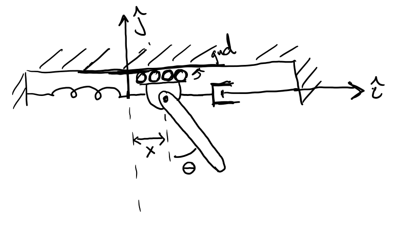
Visualize the motion

The frame_data and plot_frame functions were generated with copilot help,

Julia Assistant input,
I want to create julia animations that make this image with a spring, damper, and compound pendulum based on vectors for x position and angle theta

The resulting animation shows the damped motion with the solution created above.

Here, we can see how the coupled accelerations help to damp the pendulum's oscillations.

@gif for i in 1:length(solution)
    plot_frame(solution[1,:], solution[2,:], i)
end

Built with Julia 1.12.4 and

Latexify 0.16.10
ModelingToolkit 11.10.0
OrdinaryDiffEq 6.108.0
Plots 1.41.6

To run this tutorial locally, download this file and open it with Pluto.jl.

Dynamics

Solving the damped pendulum equations of motion

Coupled equations of motion

Compare damping terms and response

Visualize the motion