Rigid body motion with non-conservative forces
In this video, we go through the definitions of
Kinematics
Kinetics
Variational calculus
to arrive at the equations of motion for a compound pendulum with a support that has both stiffness and damping (modeled here as a spring and damper).
Kinematics
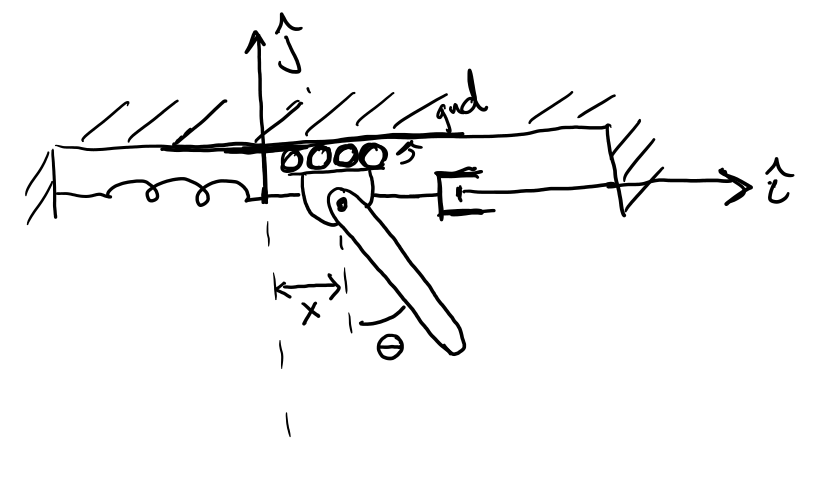
We determine the position of the pendulum is \(q_2=[x_2,~y_2,~\theta_2] = [f_1(x,~\theta),~f_2((x,~\theta)),~\theta]\)
Where the generalized coordinates are \(q = [x,~\theta]\) so the position and orientation must be written as functions of these variables. The position of the pendulum is thus
$$\mathbf{r} = (x+\frac{L}{2}\sin\theta)\hat{i} + \frac{L}{2}\sin\theta\hat{j}$$
and velocity is
$$\mathbf{v} = (\dot{x}-\frac{L}{2}\dot{\theta}\cos\theta)\hat{i} + \frac{L}{2}\dot{\theta}\cos\theta\hat{j}$$
Lagrangian of damped pendulum
The form of the Lagrangian (action, \(L=T-V\)) then results from the position and velocity definitions,
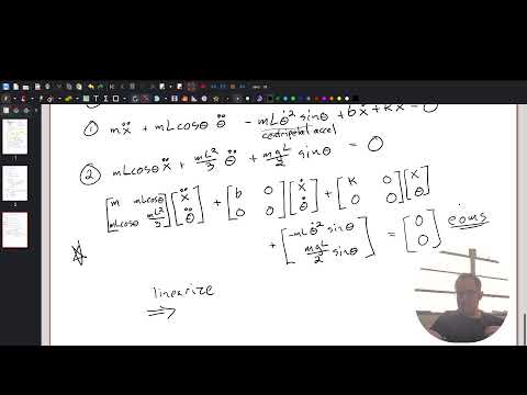
$$L = \frac{1}{2}m\left(\dot{x}^2+\frac{L^2}{3}\dot{\theta}^2 + L\dot{x}\dot{\theta}\cos\theta\right) - \frac{1}{2}kx^2 - mg\frac{L}{2}(1 - \cos\theta)$$
using Symbolics, Plots, OrdinaryDiffEq, Latexify, ModelingToolkitbegin
@independent_variables t
@parameters m=0.4 L = 1 g = 9.81 k = 0.1 b = 0.2
@variables θ(t), x(t) # θ and x are functions of time
D = Differential(t) # time derivative operator
# Define kinetic and potential energy
T = 1/2 * m *(D(x)^2 + L^2 *D(θ)^2/3 + L*D(x)*D(θ)*cos(θ))
V = 1/2*k*x^2 + m * g * L/2 * (1 - cos(θ))
# Lagrangian
Lag = T - V
end$$\begin{equation} - 0.5 ~ \left( x\left( t \right) \right)^{2} ~ k - \frac{1}{2} ~ L ~ g ~ m ~ \left( 1 - \cos\left( \theta\left( t \right) \right) \right) + 0.5 ~ \left( \left( \frac{\mathrm{d} ~ x\left( t \right)}{\mathrm{d}t} \right)^{2} + \frac{1}{3} ~ \left( \frac{\mathrm{d} ~ \theta\left( t \right)}{\mathrm{d}t} \right)^{2} ~ L^{2} + L ~ \frac{\mathrm{d} ~ x\left( t \right)}{\mathrm{d}t} ~ \frac{\mathrm{d} ~ \theta\left( t \right)}{\mathrm{d}t} ~ \cos\left( \theta\left( t \right) \right) \right) ~ m \end{equation}$$
begin
dL_dθdot = Symbolics.derivative(Lag, D(θ))
dL_dθ    = Symbolics.derivative(Lag, θ)

EL_equation_θ = expand_derivatives(D(dL_dθdot) - dL_dθ)
simplify(EL_equation_θ)
end
$$\begin{equation} \frac{1}{2} ~ L ~ g ~ m ~ \sin\left( \theta\left( t \right) \right) + 0.5 ~ L ~ m ~ \frac{\mathrm{d} ~ x\left( t \right)}{\mathrm{d}t} ~ \frac{\mathrm{d} ~ \theta\left( t \right)}{\mathrm{d}t} ~ \sin\left( \theta\left( t \right) \right) + 0.5 ~ \left( \frac{2}{3} ~ L^{2} ~ \frac{\mathrm{d}^{2} ~ \theta\left( t \right)}{\mathrm{d}t^{2}} + L ~ \frac{\mathrm{d}^{2} ~ x\left( t \right)}{\mathrm{d}t^{2}} ~ \cos\left( \theta\left( t \right) \right) - L ~ \frac{\mathrm{d} ~ x\left( t \right)}{\mathrm{d}t} ~ \frac{\mathrm{d} ~ \theta\left( t \right)}{\mathrm{d}t} ~ \sin\left( \theta\left( t \right) \right) \right) ~ m \end{equation}$$
begin
dL_dxdot = Symbolics.derivative(Lag, D(x))
dL_dx    = Symbolics.derivative(Lag, x)

EL_equation_x = expand_derivatives(D(dL_dxdot) - dL_dx)
simplify(EL_equation_x)
end
$$\begin{equation} k ~ x\left( t \right) + 0.5 ~ \left( 2 ~ \frac{\mathrm{d}^{2} ~ x\left( t \right)}{\mathrm{d}t^{2}} + L ~ \frac{\mathrm{d}^{2} ~ \theta\left( t \right)}{\mathrm{d}t^{2}} ~ \cos\left( \theta\left( t \right) \right) - \left( \frac{\mathrm{d} ~ \theta\left( t \right)}{\mathrm{d}t} \right)^{2} ~ L ~ \sin\left( \theta\left( t \right) \right) \right) ~ m \end{equation}$$
eqs_lagrange = [EL_equation_x ~ -b*D(x); EL_equation_θ ~ 0]$$\begin{align} k ~ x\left( t \right) + 0.5 ~ \left( 2 ~ \frac{\mathrm{d}^{2} ~ x\left( t \right)}{\mathrm{d}t^{2}} + L ~ \frac{\mathrm{d}^{2} ~ \theta\left( t \right)}{\mathrm{d}t^{2}} ~ \cos\left( \theta\left( t \right) \right) - \left( \frac{\mathrm{d} ~ \theta\left( t \right)}{\mathrm{d}t} \right)^{2} ~ L ~ \sin\left( \theta\left( t \right) \right) \right) ~ m &= - b ~ \frac{\mathrm{d} ~ x\left( t \right)}{\mathrm{d}t} \\ \frac{1}{2} ~ L ~ g ~ m ~ \sin\left( \theta\left( t \right) \right) + 0.5 ~ L ~ m ~ \frac{\mathrm{d} ~ x\left( t \right)}{\mathrm{d}t} ~ \frac{\mathrm{d} ~ \theta\left( t \right)}{\mathrm{d}t} ~ \sin\left( \theta\left( t \right) \right) + 0.5 ~ \left( \frac{2}{3} ~ L^{2} ~ \frac{\mathrm{d}^{2} ~ \theta\left( t \right)}{\mathrm{d}t^{2}} + L ~ \frac{\mathrm{d}^{2} ~ x\left( t \right)}{\mathrm{d}t^{2}} ~ \cos\left( \theta\left( t \right) \right) - L ~ \frac{\mathrm{d} ~ x\left( t \right)}{\mathrm{d}t} ~ \frac{\mathrm{d} ~ \theta\left( t \right)}{\mathrm{d}t} ~ \sin\left( \theta\left( t \right) \right) \right) ~ m &= 0 \end{align}$$
Built with Julia 1.12.4 and
Latexify 0.16.10ModelingToolkit 11.10.0
OrdinaryDiffEq 6.108.0
Plots 1.41.6
Symbolics 7.13.0
To run this tutorial locally, download this file and open it with Pluto.jl.