Spring-mass harmonic oscillator

Part one - setting up numerical integration

note: there's some numerical issues that come up

Part two - getting numerical integration up and running

note: ironed out some numerical issues with some hacks

In this notebook, we solve the harmonic oscillator functions for position and velocity given the differential equation,

$$\ddot{x} = -\frac{k}{m}x$$

and initial conditions

$$x_0 = 2~m$$

$$v_0 = 0~m/s$$

import OrdinaryDiffEq as ODE

using Plots

begin
    k = 100
    m = 1
    ω = sqrt(k/m)
    x0 = 2
    v0 = 0
    tspan = (0, 4*pi/ω)

    A = x0
    B = v0/ω
end

0.0

function harmonicoscillator(ddu, du, u, ω, t)
    ddu .= -ω^2 * u
end

#Pass to solvers

harmonicoscillator (generic function with 1 method)

prob = ODE.SecondOrderODEProblem(harmonicoscillator, 
                                 [v0], 
                                 [x0], 
                                 tspan, 
                                 ω)

�[38;2;86;182;194mODEProblem�[0m with uType �[38;2;86;182;194mRecursiveArrayTools.ArrayPartition{Int64, Tuple{Vector{Int64}, Vector{Int64}}}�[0m and tType �[38;2;86;182;194mFloat64�[0m. In-place: �[38;2;86;182;194mtrue�[0m
Non-trivial mass matrix: �[38;2;86;182;194mfalse�[0m
timespan: (0.0, 1.2566370614359172)
u0: ([0], [2])

sol = ODE.solve(prob, ODE.DPRKN6(), reltol = 0.000001)

retcode: Success
Interpolation: specialized 6th order interpolation
t: 92-element Vector{Float64}:
 0.0
 2.893672764104888e-7
 4.3094596785332467e-7
 1.8467328822816834e-6
 1.6004602026565272e-5
 0.00015758329346940116
 0.0014529231474200764
 ⋮
 1.1807107739201608
 1.1957894812241363
 1.211284708209366
 1.2273170540954124
 1.2440413926419842
 1.2566370614359172
u: 92-element Vector{RecursiveArrayTools.ArrayPartition{Float64, Tuple{Vector{Float64}, Vector{Float64}}}}:
 ([0.0], [2.0])
 ([-5.335295034665839e-5], [1.9999999999929348])
 ([-8.16686886350626e-5], [1.9999999999833766])
 ([-0.0003648260715007362], [1.999999999667306])
 ([-0.0031963998867704548], [1.9999999744576202])
 ([-0.03151212515060508], [1.9999975174634315])
 ([-0.2905698858976265], [1.9997889117140084])
 ⋮
 ([13.767742522230476], [1.450686959484666])
 ([11.432353471744767], [1.6410401997523374])
 ([8.762715675381127], [1.7978176037641544])
 ([5.7803484319394], [1.9146476743203364])
 ([2.512482455129625], [1.9841558195004614])
 ([4.497230755504963e-6], [1.9999999992350599])

t = sol.t  # extracting time from solution

92-element Vector{Float64}:
 0.0
 2.893672764104888e-7
 4.3094596785332467e-7
 1.8467328822816834e-6
 1.6004602026565272e-5
 0.00015758329346940116
 0.0014529231474200764
 ⋮
 1.1807107739201608
 1.1957894812241363
 1.211284708209366
 1.2273170540954124
 1.2440413926419842
 1.2566370614359172

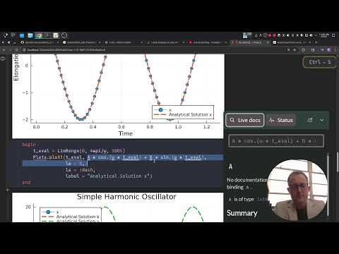
plot(sol.t, sol[2,:],
           linewidth = 1,
           marker = 'o',
           title = "Simple Harmonic Oscillator",
           xaxis = "Time", 
           yaxis = "Elongation", 
           label = "x")

begin
    t_eval = LinRange(0, 4*pi/ω, 1001)
    plot!(t_eval, A * cos.(ω * t_eval) + B * sin.(ω * t_eval), 
                lw = 3, 
                ls = :dash, 
                label = "Analytical Solution x")
end

Lagrange definition

The Principle of least action states that the difference between kinetic, $T$, and potential, $V$, energy must be minimized given the forces and constraints a system.

$$L = T-V$$

$$\min_{q(t),~\dot{q}(t)} \int_{t_1}^{t_2} T(q, \dot{q})dt$$

In this case, the kinetic and potential energy is as such

$$T = \frac{1}{2}mv(t)^2$$

$$V = \frac{1}{2}kx(t)^2$$

where $x(t)$ and $v(t)$ are functions that we just solved for with the first differential equation.

begin
    v = sol[1,:]
    x = sol[2,:]
    T = 1/2 .* m .* v.^2
    V = 1/2 .* k .* x.^2
    L = T .- V
    plot(t, T, label = "KE")
    plot!(t, V, label = "PE")
    plot!(t, L, label = "Action")
end

Integrating the action in the system

In the next step, we can use the exact equations or the numerical solutions to calculate action, $L$, and integrate over the time period we considered.

$$\int_{t_1}^{t_2} T(q, \dot{q})dt \approx \sum_{i=1..N} T(q_i,\dot{q}_i)\Delta t_i$$

where $N$ is the number of timesteps we solved and $\Delta t_i$ is the size of each timestep.

According to the principle of least action, the number we calculate should be the minimum.

function integrate_action(L, t)
    L_dt = L[1:end-1].*(t[2:end]- t[1:end-1])
    return sum(L_dt)
end

integrate_action (generic function with 1 method)

integrate_action(L, t)

-0.5880345378239729

Try your own functions

Test the math behind this claim that we have found the functions of least action. What other functions satisfy the initial conditions?

begin
    v_an = ω * (-A * sin.(ω * t) + B * cos.(ω * t))
    x_an = A * cos.(ω * t) + B * sin.(ω * t)
    
    T_an = 1/2 .* m .* v_an.^2
    V_an = 1/2 .* k .* x_an.^2
    L_an = T_an .- V_an;
end

92-element Vector{Float64}:
 -200.0
 -199.99999999665067
 -199.99999999257145
 -199.9999998635831
 -199.99998975410864
 -199.99900670104697
 -199.91556651462108
    ⋮
  -10.449355467669122
  -69.30137833647011
 -123.2148847639518
 -166.58762174537424
 -193.68745432688002
 -200.0

integrate_action(L_an, t)

-0.5880349011287564

Built with Julia 1.12.4 and

OrdinaryDiffEq 6.106.0
Plots 1.41.3

To run this tutorial locally, download this file and open it with Pluto.jl.

Dynamics